Intergenerational mobility: evidence
Section 10.3 presented a set of measures by means of which we can describe not only intra- but also intergenerational associations in a society. This section reviews evidence on such associations.
There are several earlier reviews of intergenerational income mobility. Solon (1999) reviewed intergenerational labor market with a focus on long-run earnings, whereas Solon (2002) focused on a subset of that literature, namely cross-national differences in mobility. Bjorklund andjantti (2009) built on and extended the empirical evidence assembled by Solon (1999). Black and Devereux (2011), who examined intergenerational links in income and education, emphasized evidence on causal links in intergenerational mobility. Blanden (2013) contrasted the crossnational evidence on intergenerational income, earnings, and education mobility with mobility in social class. Corak (2006, 2013a), in turn, emphasized policy implications. Corak (2013a) also drew on recent research about both socioeconomic gradients in child development and the emergence of economic persistence in labor markets.
Several recent reviews present international evidence on intergenerational income persistence in a scatter plot, plotting the estimated persistence in different countries on the vertical axis and estimated income inequality, often in the parental generation, on the horizontal, adding a linear bivariate regression line (Bjorklund and jantti, 2009; Blanden, 2013; Corak, 2013a). Labeled the “Great Gatsby” curve by the then-chairman of the U.S. Council of Economic Advisors (Krueger, 2012), such plots are interpreted to suggest countries with higher persistence are also countries with greater inequality. Figure 10.13 reproduces the most recent such graph, from Corak (2013a, Figure 1). Although the precise estimates used by different authors vary, the results are broadly similar.
The Nordic countries have low persistence and low inequality; the United States, the UK along with France and Italy, have high persistence and reasonably high inequality.There are theoretical models that can account for the positive association between inequality and persistence. For instance, in Solon’s (2004) version of the Becker and Tomes (1979, 1986) model, the factors that drive intergenerational persistence, such as the heritability of human capital endowments, the returns to education, and the progressivity of public education expenditure, affect cross-sectional inequality with the same signs. In Hassler et al.’s (2007) model, which examines links between inequality and mobility under different kinds of labor market institutions, some institutional arrangements have mobility and inequality being inversely related (and hence persistence and inequality positively correlated). Checchi et al.’s (1999) model of beliefs about own ability, educational choice and mobility can also generate positive as well as negative associations between inequality and mobility depending on the model parameters. As we shall see, however, it is far from clear that intergenerational persistence and inequality are, in fact, as clearly positively correlated as Figure 10.13 suggests.
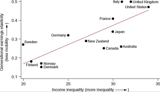
Figure 10.13 The Great Gatsby curve: the relationship between intergenerational earnings persistence and cross-sectional income inequality. Note: Income inequality is measured by the Gini coefficient of disposable household income in 1985 taken from the OECD. Persistence is measured as the Beta of parental and son earnings. Sons are born in early 1960s, and outcomes for them are measured in late 1990s. See Corak (2013a,b) for further detail. Source: Corak (2013a, Figure 1).
This part of the chapter proceeds as follows. In Section 10.5.1, we discuss data requirements and special problems that come up in estimating intergenerational and family associations.
In Section 10.5.2, we review studies of intergenerational persistence and mobility in the United States. The focus on this country is motivated, as in the intragen- erational mobility case, by the sheer amount of evidence about mobility in the United States relative to that in other countries. First, we examine evidence on the level of the intergenerational elasticity (IGE) of earnings or income—first for father-son pairs, and then widen the scope to look at broader pairings of parents and offspring—and then examine evidence about trends in the IGE over time. (The IGE is the Beta measure discussed in Section 10.3; we use both terms interchangeably in this section.) We then examine evidence that is based on measures that go beyond the simple log-linear Galtonian regression Beta (IGE), product-moment correlation coefficient r: for example, quantile regressions, transition matrices, nonparametric conditional mean functions. In Section 10.5.3, we examine evidence on intergenerational mobility from other countries, following the same structure as for the United States. In Section 10.5.4, we examine evidence on another way to measure the importance of family background, the sibling correlation; and in Section 10.5.5, we discuss other approaches to intergenerational mobility, old and new. Section 10.5.6 concludes.10.5.1 Data and Issues of Empirical Implementation
As discussed in Section 10.4.1, any study of income mobility faces three “W” issues: mobility of What, among Whom, and When? For intergenerational mobility, each question must be answered twice, once in each of the parental and offspring generations. As with intragenerational mobility, researchers’ choices are constrained with the available data.
At one level, just as with intragenerational income mobility, mobility of “What” refers to the income concept that is used. The overwhelming majority of studies we review use the labor market earnings of the parent and the offspring with several variations, discussed in Section 10.4.1.
Other choices might add nonlabor income sources from the market such as capital income to measure factor or market income. If the goal is to examine the intergenerational association ofliving standards, it would make sense to study disposable income (i.e., to add public transfers and deduct income taxes paid). It would seem reasonable to have identical answers to the “What” question in both generations. It is frequently the case that available data do not support such a choice; it is not unusual for “income” to be family income in the parental generation and to be earnings in the offspring generation.[628]The aim of early research on this topic was to measure the intergenerational association of “permanent” income, which was believed to be captured quite well by labor market earnings. It has long been recognized (see Atkinson, 1981b) that short-run income measures are different from longer-run measures because of transitory fluctuations, and that the associations sought were those of the more stable or permanent measures ofliving standards.
As with intragenerational mobility, “Whom” refers to the definition of the incomereceiving unit in both the parent and child generation. Most studies that are modeled on Solon (1992) examine mobility of father-son pairs, ignoring the incomes of other household members. Many departures from this are due to data-related reasons. For instance, studies such as that of Zimmerman (1992), which relies on data from the U.S. National Longitudinal Survey of Youth (NLSY), uses family income in the parental generation, as that is the only income concept available in that data source.[629]
The Whom question becomes more complex when the intergenerational associations of women’s incomes are studied and compared with those of men. Over the last four to five decades, women’s labor market attachment has increased substantially in most developed nations, with female labor force participation rates increasingly resembling those of men.
However, around the age commonly believed to be appropriate for measuring men’s long-run income (around age 40), women often have breaks from employment due to childbirth and child care. Studies that examine women’s intergenerational mobility are more likely to examine family or household income as a better gauge of their living standard than individual incomes. Comparing mobility across men and women would then naturally also need to examine family or household income for men (Chadwick and Solon, 2002; Raaum et al., 2007).There is an added dimension to the Whom question, namely the nature of the parentoffspring relationship. In the early intergenerational studies of Atkinson (1981b), Solon (1992), and Zimmerman (1992), the parent-child association was more or less driven by the survey design—“children” were the children of the sample parents who were followed up in adulthood. However, children can have multiple parents—stepparents, adoptive and foster parents in addition to birth parents. Common choices are to restrict the population to those parent-offspring pairs where the offspring was observed as living with the parent at some age, say 10 or 16, or to birth parents. One aspect of this Whom dimension is the role of separated families. Should one focus on associations of offspring income with the head in lone-parent families or on father-child associations? Some studies, especially based on register data, have examined the sensitivity of the population of parent-child relationships and found differences across definitions and family types to be relatively small.[630]
As with the two other “W” questions, the When question for intergenerational mobility analysis is mostly a superset of that for intragenerational mobility. Most of the same questions addressed in Section 10.4.1 need to be resolved for both the parent and offspring generations. The underlying data record income for a specific period: often annual income data but in some cases “current” income data are available.
But, in contrast to the case ofintra- generational mobility, shorter-run fluctuations are noise that make more difficult the uncovering of the more interesting underlying longer-run incomes. This leads directly to the issue of over what periods, and over what ages, incomes should be studied (and aggregated) to give reasonable measurements of longer-run economic status. And if, due to data limitations, ideal measurements cannot be made, how are mobility measurements affected? The two main issues that have been addressed are transitory variation in observed income measures, and “life cycle” bias (Jenkins, 1987; Grawe, 2006). We discuss these in turn.Since at least Atkinson (1981b), it has been recognized that transitory errors in parental income lead to an errors-in-variables (downward) inconsistency in the estimated intergenerational elasticity. Since the seminal paper to empirically address this issue (Solon, 1992), many studies have exploited this finding.[631] Solon’s estimate of intergenerational persistence for the United States, based on averages across 5 years of parental income, resulted in point estimates of Beta that are between 10% and 70% larger than the estimates derived using a single year of parental income.
Recent work on so-called generalized-errors-in-variables (GEIV) model calls into question the assumption that transitory income variations have the same properties as classical measurement errors (Bohlmark and Lindquist, 2006; Haider and Solon, 2006). The GEIV model for the annual income process of an individual in family i in generation j (=Offspring, Parent) at age t relates permanent income y and transitory errors v to annual or current income by (Haider and Solon, 2006)

The key advance here is the introduction of the age-dependent parameter #955;, which “loads” underlying permanent income onto annual income and is hypothesized to be lower than one early in the life cycle, equal to one at some point, and higher than one thereafter. Note that we allow for the #955; parameters to differ across generations.[632] [633] The measurement error model in Equation (10.16) is the same as the classical measurement error model if (i) #955;jt ? 1, and (ii) the random fluctuations v are orthogonal to true long-run income (y ? v), and the vs are identically and independently distributed within a generation. An estimate of the IGE #946; using annual incomes for both parents and children has the probability limit However, the age- or time-dependent factor loading #955;jt leads to two additional sources of bias in the IGE, namely the age/time point at which child incomes is The probability limit of the correlation coefficient depends on the #952; in both generations, on the ratio of the observed standard deviation to that of long-run income in both generations, as well, of course, on the true r. Empirical evidence from both the United States and Sweden on the age profile of #955;t based on the GEIV model, suggests that earnings early in life (even abstracting from a population age-earnings profile) are a downward-inconsistent measure of lifetime earnings and later in life an upward-inconsistent measure (Bohlmark and Lindquist, 2006; Haider and Solon, 2006). Around age 40, at least for men in both the United States and Sweden, #955;t #8776; 1 in which case deviations from a multiyear average are approximately classical, thus lending themselves to the analysis of intergenerational association oflong- run income under the assumption that the #955;s in both generations are approximately equal, i.e., #955;pt#8776;#955;#952;t (or at least that they were equal at about the same age). Grawe (2006), building on insights in Jenkins (1987), examined the extent of both attenuation and life cycle bias in Betas estimated in several different countries and data sets. He found, using data for Canada, Germany, and the United States, that life cycle biases in fathers’ age are an important source of bias and proposed several rules of thumb to diminish it: either to use points in time at which measurement errors are roughly classical, as suggested earlier, or at least to use observations on income for parents and children at similar points in their life cycle. There are several caveats, however. First, as implied earlier, the #955;s may well change from one generation to the next. Second, the #955;s that apply to, say, earnings, may differ from those that apply to, say, disposable household income. Third, the #955;s that apply to men may be quite different than those that apply to women depending, for instance, on patterns of labor force withdrawal and reentry due to child bearing. Finally, the #955;s can be quite different in different countries. Without access to estimates of these, cross-country differences in the IGEs can be driven not by differences in the underlying #946;s but by different values of #955;#952;t and #952;ps, even if the ages at which incomes are measured are kept 65 constant. It may be interesting to know how large the bias in Beta or r is in a given population. However, we are often interested in comparing these parameters in two different populations, for example, across time in a country, or between two countries. Denoting the two populations by A and B and focusing on Beta, and assuming for simplicity we are measuring both parents and offspring at the same ages, we have 65 Moreover, Nybom and Stuhler (2011) used nearly complete actual lifetime incomes for both fathers and sons. By comparing regression coefficients based on multiyear averages of sons’ income with thatbased on their full lifetime incomes, they found that the biases in the intergenerational elasticity estimates are still quite considerable. This may mean that more complex models that link short-run to “permanent” income need to be explored. the sign of their difference without bias (but cannot know its size unless we know #955; and #952;), or we can estimate their ratio. The almost exclusive focus on permanent income (which, in some sense, involves both the What and When questions) can be questioned in light of the more complicated measurement models that link short-run to long-run income. The focus on permanent income is based on the notion that differences between short- and long-run income are transitory and largely classical, i.e., positive and negative shocks are roughly as likely (low or not autocorrelation), and the magnitude of the shocks does not vary by either permanent income or other characteristics (shocks are homoscedastic and orthogonal to permanent income). If capital markets are well functioning and individuals have a fair idea of what their permanent income is (so they know if they have been hit by a negative or positive shock), they smooth their consumption by relying on saving and borrowing. These demanding conditions would justify the focus on permanent income (see the discussion in Section 10.2). In this view, it is permanent income, not short-run fluctuations, that best captures the distribution of well-being. It follows that, if the assumptions are violated, even short-run fluctuations are interesting from a well-being perspective. Jantti and Lindahl (2012) demonstrated that income volatility in Sweden is strongly but nonmonotonically associated with the level of long-run income. Moreover, analysis of intergenerational associations in income suggests that not only long-run incomes but also income volatility is associated across generations (Jantti and Lindahl, 2012; Shore, 2011). Thus, a focus on long-run incomes alone probably understates the extent to which economic well-being is associated across generations. Before we discuss commonly used data sources for intergenerational analysis, we point to an additional complication in interpreting the evidence. The most commonly used measure of intergenerational mobility is the persistence as measured by Beta (the IGE). Arguably, we would like to abstract from the marginal distribution of offspring and use the correlation, r, related to Beta by the ratio of parental to offspring standard deviation (see Equation 10.4). In steady state, the two are equal but, when inequality increases (decreases) across generations, r is lower (higher) than Beta. Extra care should then be taken in comparing Betas across countries, as different Betas may be consistent with the same, or at least more similar r, depending on how marginal distributions have changed across generations in the two countries. Bjorklund andjantti (2009) cited evidence that suggests the ratio #963;p#8725;#963;o in the United States is less than one—inequality increased—and in Sweden greater than one—inequality decreased—suggesting the difference in r is likely to be less than that in the Betas. (Note, however, that it is only changes in inequality in the marginal distributions that are controlled for, and in a particular way.) Suitable data for intergenerational analysis need to meet two basic criteria. The data need to be able to identify and link parent-child pairs.[634] They need to include measurements of the incomes in both generations at comparable points in the life cycle and preferably multiple such measurements to allow for the effect of measurement errors. Three main types of data are used. Many studies rely on longitudinal household surveys that have been running long enough to allow for the offspring to be observed living with their parent(s) as a child or youth and then followed up as adults, having often formed households of their own. These data sources, discussed in greater detail in Section 10.4.1, include the U.S. PSID and the German SOEP. The UK BHPS has only recently been used for intergenerational analysis. Cohort studies are another type of data that are commonly used for intergenerational analysis. Such data sets, including the U.S. National Longitudinal Study of Youth (NLSY) and the UK National Child Development Study (NCDS; cohort of 1958) and British Cohort Study (BCS, cohort of 1970), have been specifically designed to collect data on children and follow them across time as they grow older. The income and other information used are mostly gathered through interviews with the parents and children in such studies, and the parent-child link is ascertained from both information about both birth and living arrangements. A variation of the survey-based approach was taken in the UK, where Atkinson (1981b, 1983), using data originally collected by Rowntree and Lavers (1951) for the study of cross-sectional poverty in York, built an intergenerational data set by interviewing the adult children of the original survey households, creating a longitudinal data set from what was originally a cross-sectional data set. Register-based data sets are another important source of data. Such data, which underlie intergenerational mobility estimates in Canada and the Nordic countries, and increasingly also in the United States, rely on administrative records, often drawn from data originally collected for purposes of taxation or Social Security, to measure income, and identify parent-child links based either on administrative records that link parents to children or on census data.[635] The key to the use of such data is the use of personal identifiers and the presence of a reliable parent-child link. A third approach to data is to use synthetic parent-child links. One way to do this is to use two-sample methods (i.e., to estimate Beta using empirical moments based on different data sets). This requires a sample of “parents” to provide information on the unconditional distribution of income in the parental generation and of the distribution conditional on a few key predictors of income, as well as a sample of “offspring” to provide information on both their income distribution and on the predictors for their parents. Two-sample methods, first used in the intergenerational context by Bjorklund and Jantti (1997) for a comparison of the United States and Sweden, have later been used in several countries, including Britain, Italy, France, Brazil, and Australia.6 Each of these three types of data is subject to measurement challenges (see Section 10.4). Measurement errors in income and other data used in the analysis are an issue, and not only in survey- but also in register-based sources, although the nature of the errors are likely different (e.g., recall error in survey data and underreporting due to tax evasion in register data).[636] [637] Attrition, especially selective attrition, is a concern in longitudinal surveys, a problem that may be compounded in intergenerational follow-up. The reliability of the identification and linking of parents and children is a concern when that is done using administrative data. Before we delve into the evidence, we should note that the overwhelming majority of studies, in the United States as well as in other countries estimate elasticities (i.e., estimates of the Beta measure discussed in Section 10.3). When correlations are available (either directly, reported by the authors, or derived using Equation 10.4 based on Betas and the standard deviations), they are product-moment (Pearson) rather than rank (Spearman) correlations. Fully controlling for the marginal distributions would require the latter. Moreover, we are unaware of any study that explicitly recognizes the implications of the GEIV model for estimated elasticities that attempts to control for those effects. One reason most analysts may estimate Betas rather than Pearson or Spearman correlation coefficients, or transition matrices, is convenience: controlling for systematic life cycle effects in both generations is simple in a multiple regression framework. Moreover, the impact of transitory errors, when classical, is well understood and simple to mitigate. Estimation of the Pearson correlation is subject to the same errors-in-variables inconsistency as the Beta, but transitory errors in both offspring and parent income cause r to be underestimated, so reducing the inconsistency requires time-averaging income in both generations. Transitory errors lead to inconsistent estimates of rank correlations also. O’Neill et al. (2007), who presented simulation evidence based on bivariate normal distributed parent-offspring income that are subject to a range of different kinds of measurement error, suggest robustly that intergenerational persistence is underestimated and mobility overestimated in the presence of measurement error. Finally, in many cases, Beta and r are estimated using instrumental variables, often using sample moments from different samples. These techniques are well understood in moment-based estimation, but less so for rank correlations and nonparametric techniques. 10.5.2 Intergenerational Persistence in the United States Although there are many studies of intergenerational mobility in the United States as well as in other countries, the literature is characterized by a surprising number of omissions. For instance, we have been unable to locate transition matrices for different cohorts of parent-child pairs, so we are unable to examine the change across time in mobility using the dominance approach.[638] Most U.S. researchers report only Betas, not r or rank correlations, so standardization for changes in the marginal distribution of earnings or income is incomplete at best. And yet this is a period in which there have been pronounced increases in inequality in the United States (and many other countries). By the late 1980s, two longitudinal data sets in the United States, the Panel Study of Income Dynamics (PSID) and the National Longitudinal Study of Youth (NLSY) had been running for sufficiently long to allow the study of the incomes of parents and children at economically active ages. Around that time, three papers were published in reasonably close succession that made use of these data, by Solon (1992), Zimmerman (1992), and Altonji and Dunn (1991). The papers by Solon (1992) and Zimmerman (1992), which appeared prominently in the same issue of the American Economic Review, made two major contributions.[639] First, they pointed out some of the statistical problems involved in estimating the relationship between “long-run” incomes of members of the same family. Most earlier studies used single-year measures of permanent earnings and were based on nonrepresentative, homogeneous samples. Their analyses suggested that the estimates of intergenerational correlations in previous studies most likely were considerably downward biased. By using multiple years of fathers’ earnings, this downward bias could be reduced. Solon also presented an estimator that most likely overestimates the correlation and thus produced a range within which the true correlation must lie. Second, their results suggested Betas between fathers’ and sons’ long-run incomes as high as 0.4 or 0.5, numbers that are much larger than those in the previous studies surveyed by Becker and Tomes (1986). Solon and Zimmerman obtained similar results using two different data sets, which lends additional credibility to their findings. Solon (1992) also estimated the correlation by use of an instrumental variables (IV) method, arguing that this produces an upward inconsistent estimate of Beta. The argument, in brief, is to treat parental education as an omitted variable, but also to use parental education as an instrument, so it is an invalid instrument. Ifthe true direct effect of parental education is positive and it is positively correlated with parental income, such an IV estimate produces an overestimate of the intergenerational income elasticity. Thus, the OLS estimator using time-averaged parental income underestimates and the IV estimator overestimates the elasticity, bounding the parameter from below and above. Moreover, in pointing to the possibility of using an IV estimator, Solon (1992) also opened the door to estimating elasticities, reliably as it turned out, in cases where actual father-son pairs are unavailable.[640] Mazumder (2005b), using earnings information from the U.S. Social Security Administration (SSA), examined intergenerational earnings Betas for U.S. sons and daughters with respect to fathers’ earnings. His focus is on variations in the number of years across which fathers’ earnings are averaged, along with several other measurement issues such as whether or not to require fathers to have positive earnings in all years, if zero earnings due to noncoverage of Social Security by registers are imputed or not, as well as whether or not zero earning offspring are included in the analysis. The results demonstrate, among other things, that attenuation from transitory variation in earnings remains substantial even after averaging fathers’ earnings over up to 16 years, especially if transitory errors are characterized by autocorrelated errors. In a striking demonstration of the the impact of averaging across multiple years of parental income, Mazumder (2005b, Table 4) reported an elasticity of 0.253 (se 0.043) when only 2 years (1984-1985) of fathers’ incomes are used, increasing to 0.553 (se 0.099) and 0.613 (se 0.096) when averages across 1976-1985 and 1970-1985 are used, instead. The U.S. estimates he reported thus encompass the majority of the estimates reported in Figure 10.13, excluding only Peru at the top end and Canada, Finland, Norway, and Denmark at the low end. Note, however, that in extending the number of periods over which fathers’ income is averaged conflates two types of effects, namely transitory errors (whose variance is reduced) and life cycle effects (which become averaged). In the absence of estimates of #955;ps and #952;ps, it is hard to tell which of these is empirically responsible for the change in the elasticity. Dahl and DeLeire (2008), also using data from the SSA but with data on noncovered years as well and using even longer time spans for fathers’ earnings than Mazumder (2005b), estimated Betas for father-son and father-daughters pairs. The father-son estimates vary between 0.259 and 0.632, spanning, again, much of the observed range in the cross-country evidence on display in Figure 10.13. The father-daughter Betas range from —0.041 (which is not significantly different from zero) to 0.269. Naga (2002) used father-son pairs observed at the same point in the life cycle and estimated elasticities using three methods—OLS on time-averaged data, IV, and a MIMIC latent variable estimator—and found elasticities that range from 0.297 to 0.7. Chadwick and Solon (2002), Minicozzi (2002), and Fertig (2003) also examined Betas for women. Chadwick and Solon (2002) highlighted the importance of using family income when comparing Betas for men and women (in which case they are quite similar; when using individual earnings, Betas for women tend to be much lower). The sensitivity of Betas to sample selection rules was examined by Couch and Lillard (1998) and Minicozzi (2003). In both of those papers, sample selection issues were found to be very important for the Betas. Hertz (2005) examined racial differences in the elasticity. Estimates of Beta for the United States can also often be found in research that is either comparative or primarily about other mobility in other countries, Examples include the studies of Germany by Couch and Dunn (1997), Australia by Leigh (2007), Sweden by Bjorklund andjantti (1997), and Singapore by Ng et al. (2009). Two U.S. papers that drew attention early on to the possibility that estimates ofinter- generational persistence may be subject to not only attenuation inconsistency from transitory errors in fathers’ earnings or income, but also to life cycle effects in the offspring generation, were Buron (1994) and Reville (1995). Instead of adjusting for the average life cycle effects, Buron (1994) allowed earnings profiles to vary across demographic groups, which leads to a higher estimated persistence than when using the same adjustment. Reville (1995) in turn investigated how varying the age and outcome year of sons changes the estimated persistence. For instance, by following the same cohort of offspring as they age from 26-30 to 34-38 and using a 4-year average of their earnings (keeping father’s earnings constant), the Pearson correlation r increases from 0.296 to 0.423 (Reville, 1995, Table 5). Hertz (2007), Lee and Solon (2009), Gouskova et al. (2010), and Chau (2012) all try to take into account biases from both transitory errors and life cycle effects. Gouskova et al. (2010), applying the insights of both Haider and Solon (2006) and Grawe (2006), estimated earnings elasticities for father-son pairs using data from the PSID, where the fathers and sons are of the same age. Using age ranges 25-34, 35-44, and 45-54, regressing a 3-year average of sons’ earnings on a 5-year average of fathers’ earnings, they found elasticities of 0.29, 0.41, and 0.42, respectively. These estimates, especially the low value for the 25-34 age range, are consistent with the patterns for #955; in Haider and Solon (2006). Another recent study considering the implications of the results in Haider and Solon (2006) and Chau (2012) models the income processes ofboth fathers and sons using heterogeneous growth profiles and autocorrelated errors. Intergenerational elasticities are then estimated based on data simulated using the parameter estimates. The U.S. estimates, based on PSID data, show an estimate of Beta of 0.392, but elasticities are as high as 0.662 when the earnings processes of sons and fathers are allowed to be different. Muller (2010) tackled another complication with estimating the measurement of permanent income, namely if the elasticity varies because of shocks to parental income that take place when the offspring was living in the parental home. Parental income earned in childhood years is associated with much higher elasticities than either before the child was born or after he had left home, a result that is broadly robust with respect to standardizing the stage of the life cycle at which incomes are measured in the two generations. The results are consistent with the view that transitory shocks in childhood do affect offspring income. Although the purpose of the literature on intergenerational mobility reviewed here is not to uncover causal effects of income, this finding lends weight to the view, discussed in Section 10.5.1, that income risk may also be intergener- ationally correlated. Trends over time in intergenerational mobility in the United States, as measured by changes in Beta, have been estimated by Hertz (2007), Mayer and Lopoo (2005), Lee and Solon (2009), and, using two-sample methods, by Aaronson and Mazumder (2008). We show a selection of estimates in Figure 10.14, indexed by the birth year of the offspring, ranging from men born in the 1920s to men and women born in the early 1970s. The elasticities are evaluated at somewhat different ages, but the picture that emerges is one that suggests little systematic trend among men, with the possible exception that persistence may have increased among men from the 1940s to 1960s, mainly on display in the Aaronson and Mazumder (2008) estimates and weakly supported by both Hertz (2007) and Lee and Solon (2009). The estimates for women in Hertz (2007) and Lee and Solon (2009) suggest increasing persistence for the early cohorts but little change from around 1960 onward. The differences across studies suggest care must be taken in interpreting trends based on but a few data points and sets of definitions. The large confidence intervals around each point estimate also highlight the importance of statistical inference. Indeed, all the confidence intervals in the series from Hertz (2007), Lee and Solon (2009), and Mayer and Lopoo (2005) overlap. Although this does not mean there cannot be significant differences between point estimates, it does warrant some caution. The IGE (Beta) is related to a “global” log-linear regression, forcing the slope of the conditional expectation of offspring log income to be a linear function of parent log income. There are many ways to relax the assumption that the slope is the same everywhere. Differences in the slope at different levels of parental income can be motivated by theoretical concerns. A commonly cited concern is the potential presence of borrowing constraints with respect to parental investments in child human capital (Becker and Tomes, 1986; Bratsberg et al., 2007; Grawe, 2004b). Bratsberg et al. (2007) fit a polynomial in parental income to the data for the United States drawn from the NLSY to allow for a flexible shape between offspring and parental income. They found that a second-order polynomial in parental income provides a reasonable fit for U.S. data. The IGE based on a log-log regression is 0.542, whereas those based on the polynomial imply elasticities of 0.489, 0.575, and 0.646 at the 10th, 50th, and 90th percentiles of parental income, respectively. Couch and Lillard (2004) demonstrated that these results are highly sensitive to the procedure applied. Using both second- and third-order Figure 10.14 (See legend on next page) polynomials in both the log and the level of parental income, they estimated elasticities in the first, third, and fifth quintile groups of fathers’ income to be 0.124, 0.234, and 0.292 using a quadratic, and 0.219, 0.230, and 0.171 for the cubic polynomial, compared to 0.158 in the log-log. Thus, using the second-order polynomial, elasticities increase monotonically across fathers’ income but, using the third-order polynomial, they increase to decline at higher levels. Another option is to estimate the conditional mean (and, by implication, its slope) nonparametrically, for instance using kernel regression. The elasticity is a measure of average persistence of income rather than of mobility. In other words, the regression coefficient on father’s log (permanent) earnings tells us how closely related, on average, an offspring’s economic status is to that of his or her parent. It is quite possible for two distributions to have highly similar average persistence, but for one to have substantially more mobility around that average persistence. The elasticity can thus be the same, but arguably the distribution with a greater residual variation— variability around the average persistence—is the one with greater mobility (see the discussion of the Gottschalk and Moffitt “BPEA” measure in Section 10.3). Moreover, two distributions with the same regression slope may have quite different, and varying, conditional variances around that slope. For instance, a distribution with a “bulge” in the variance at low levels of fathers’ earnings, that is, a pear-shaped bivariate distribution, will exhibit relatively more mobility at the low end of the distribution than will a distribution with a constant conditional variance. One approach is to examine both the regression coefficients and residual variances. Other approaches, such as nonparametric bivariate density estimates, similar to Figure 10.4 in the intragenerational case in Section 10.3, would in principle be available (see, e.g., Bowles and Gintis, 2002). Very few studies take that route, however. Quantile regression (Koenker, 2005) can also be used to examine the conditional distribution of offspring income, conditioned on parental income. Although the slopes of the conditional quantiles of offspring income can be of interest in and of themselves, we tend to find what they say about the full conditional distribution of greater interest than the slopes of individual quantiles (cf.the discussion of this in Section 10.3.3). In the prototypical homoscedastic regression, where the variance (or indeed, any higher moments) of the Figure 10.14 Trends in U.S. intergenerational income persistence. Note: The estimates in Lee and Solon (2009) are the elasticities for different outcome years at age 40, presented here by subtracting 40 from the outcome year and are derived using a 3-year average of parental income. Mayer and Lopoo (2005) estimate elasticities for 4-year birth cohorts, which are centered here, observe offspring at age 30, and use a 7-year average of parental income (at ages 19-25). Hertz (2007) presents elasticities at age 25 and uses a 3-year average of income. His estimates further control for panel attrition. Aaronson and Mazumder (2008) uses two-sample methods applied to (IPUMS) census data, with elasticities applying to 35- to 44-year-olds, here centered at age 40. Source: Aaronson and Mazumder (2008, Table 1, column 6), Hertz (2007, Table 4), Mayer and Lopoo (2005, Table A1), and Lee and Solon (2009, Table 1). residual does not depend on the explanatory variable, the quantile regression slopes should all be straight lines with slopes equal to the conditional mean and median. Deviations from these patterns are informative of variations in the shape of the conditional distribution. Eide and Showalter (1999) estimated quantile regressions for several percentiles using PSID data on father-son pairs where the sons are 25-34 years old, using a 3-year average of parental income and 7-year average of sons’ earnings. They found a Beta of 0.34 and slopes of the conditional quantiles with respect to parental income of 0.77 at the 5th percentile, 0.47 at the 10th percentile, 0.37 at the 50th percentile (median), 0.17 at the 90th percentile, and 0.19 at the 95th percentile. That is, they (mostly) find the slope to be decreasing in the percentile but also that the Beta is lower than the slopes of the quantiles up to the 75th percentile.[641] Conditional quantiles can be combined with nonparametric techniques to allow for the slope to change flexibly. We illustrate this in Figure 10.15 from Lee et al. (2009), who used PSID data for U.S. sons and fathers to nonparametrically estimate the conditional quantiles of sons’ income conditioned on fathers. We can see that the slopes of lower quantiles tend to be steeper at low parental income than for the higher quantiles and that the slopes tend to level of as parental income increases. Figure 10.15 Intergenerational income persistence: nonparametric quantile regression for U.S. father- son pairs. Note: Estimates based on PSID father-son pairs as prepared by Minicozzi (2003). Sons' income is the average of labor income at ages 28 and 29, and parental income is predicted parental income as defined by Minicozzi (2003). Source: Lee et al. (2009, Figure 1). 73 Asymmetries in intergenerational mobility can be straightforwardly described using transition matrices, a simple but underused device for illustrating intergenerational mobility. In allowing for fairly general patterns of mobility, mobility or transition matrices offer the additional advantage of allowing for asymmetric patterns, for example more mobility at the top than at the bottom. To illustrate, we show in panel A of Table 10.5, a decile transition matrix for U.S. fathers and sons. The cell entries show, for each decile group of origin (i.e., fathers’ decile group), the percentage of sons in each destination decile group. Specific aspects of the transition matrix tend to be highlighted. For instance, the main diagonal shows the percentage of sons who remain in their father’s decile group. One descriptive statistic is the sum of the main diagonal probabilities (the matrix trace), in this case 165. With ten income classes, there is origin independence if each entry in the table is 10%, which implies an average “excess” immobility relative to origin independence of 6.5% points. Conversely, 83.5% of U.S. sons are in a different decile group than their fathers. The Normalized Trace index (Shorrocks, 1978b) for this matrix is (10 — 165/100)/(10 — 1) = 0.93. The corner probabilities are often of special interest also. In this case, 22% of the sons of the poorest 10th of fathers are in the poorest 10th themselves, whereas 26% of the sons of the richest 10th of fathers are in the richest 10th. Conversely, upward mobility from the lowest 10th is 100 — 22 = 78%, and downward mobility from the highest 10th is 100 — 26 = 74%. By contrast, 7% of sons of poorest fathers and 3% of the richest end up in the top and bottom decile groups, respectively. Somewhat to our surprise, we are unable to illustrate an application of dominance analysis to examine the change across cohorts in U.S. intergenerational mobility. We are unaware of a comparable transition matrix for a later or earlier cohort. A final observation can be made regarding the “shape” of the transition matrix. Transition matrices for bivariate normal data, such as the simulated data in O’Neill et al. (2007) or the illustrations of the consequences of different r in Bjorklund and Jantti (1997), are symmetric. For instance, the two corners on the main diagonal are equal as are the corners on the antidiagonal, and the upper triangle is the mirror of the lower triangle. The U.S. father-son transition matrix clearly exhibits very little symmetry of this sort. The lack of symmetry implies that both mobility and persistence may be different across the distribution, and of course that the data are unlikely to be well described by a bivariate log normal distribution. Recently, Bhattacharya and Mazumder (2011) proposed a set of measures based on the bivariate percentile distribution, focusing specifically on upward and downward mobility relative to a parameter #964; that specifies the number of percentiles one needs to move up to be considered upward mobile, illustrating their approach by comparing mobility differences between racial groups in the United States using data on men from the NLSY. Whites are found to be distinctly more likely to move upward than blacks. Table 10.5 Intergenerational decile transition matrices for earnings, father-son pairs, Canada and the United States Note: The cell entries show, for each decile group origin (referring to fathers), the percentage of sons in each destination decile group. U.S. estimates are based on SIPP matched to Social Security earnings. Fathers' earnings are averaged across 1979—1985 and sons' across 1995—1998. Canadian data are basedon tax records. Fathers' earnings are averagedacross 1978—1982 and sons' earnings across 1993—1995. Source: Mazumder (2005a, Table 2.2) and Corak and Heisz (1999, Table 6). 10.5.3 Cross-National Comparative Evidence on Intergenerational Associations We now turn to examining evidence on intergenerational income mobility in other (mostly rich) countries. To illustrate the importance of how mobility is measured for cross-country rankings, we start this subsection by reporting results from two recent papers, each of which compares three countries. Corak et al. (2013) compared earnings mobility between fathers and sons in Canada, Sweden, and the United States. Their focus is on comparing upward and downward mobility, but we rely here on their three estimates of persistence: Beta (IGE), the Pearson correlation r, and the Spearman rank correlation are reported in Table 10.6 along with the ranking of the three countries in each case. The estimated Betas are in line with those found in previous research and show intergenerational income persistence to be the greatest in the United States, followed by Canada and Sweden. The ranking by the product-moment correlation r is the same, but now the U.S. point estimate is much closer to those of Canada and Sweden. By contrast, according to the rank correlations, Canada has the lowest persistence, and Sweden and the United States are tied. This, arguably the preferred scalar index of persistence (as it most clearly abstracts from differences in marginal distributions), suggests a very different ordering of countries with respect to intergenerational mobility than that on display in the “Great Gatsby” curve of Figure 10.13. Eberharter (2013) estimated persistence in terms of Betas for disposable income among men and women in Germany, the UK, and the United States, using data from the U.S. PSID, the German SOEP, and the UK BHPS. The elasticity estimates are reported in the left panel of Figure 10.16 together with the 95% confidence intervals. This is a rare study because it presents estimates for several countries using measures of disposable income. It is also unusual to pool sons and daughters, although that choice is arguably well motivated when the purpose is to examine the persistence in living standards. Table 10.6 Intergenerational earnings mobility in Canada, Sweden and the United States: Beta, r, and the rank correlation Note: Canadian estimates rely on tax records. Father's earnings are a 5-year average and son's a 3-year average 1997-1999 when they were 31-36 years old. Swedish estimates, also based on tax records for earnings, rely for fathers on 20 years of earnings data measured at ages 30-60 and for sons on an 11-year average across ages 30-40. The U.S. estimates stem from the Survey of Income and Program Participation panels using earnings from Social Security records. Fathers' earnings are a 9-year average between 1979 and 1986 when they were 30-60 years old. Sons' earnings are a 5-year average between 2003 and 2007 in years they were at least 28 years old. Source: Corak et al. (2013, pp. 10-11). Although Eberharter (2013) did not report rank correlations, these results bring out quite forcefully the importance of being wary of changes in marginal distributions across the cohorts, especially when comparing estimates from different countries.[642] As can be seen by comparing the left panel of Figure 10.16, which plots the elasticities, with the right panel, which reports the implied (Pearson) correlations r, the results are dramatically different in the two cases. The United States has a substantially higher elasticity than either Germany or the UK (0.68 as opposed to 0.48 and 0.50), but when we derive Figure 10.16 Intergenerational persistence of disposable Incomeielasticitiesversuscorrelations. Note: Error bars show 95% confidence intervals. Estimates are for posttax, posttransfer income for all individuals (for sons and daughters combined). Offspring incomes are observed for those older than 24 who are out of full-time education and are averaged across 2005-2009 (Germany), 2003-2007 (USA), and 2004-2008 (UK). Parental income are observed as offspring were 14-20 years old and are averaged across 1988-1992 (Germany), 1987-1991 (USA), and 1991-1995 (UK). Eberharter (2013) reports standard deviations in parental and offspring generations for full samples rather than the estimation samples, so the estimated implied correlations, obtained using p frac14; sP/sOb are approximate only. Source: Authors' elaborations based on Eberharter (2013, Tables 1 and 2). 74 the correlations, the UK has a correlation that is higher than that in the United States, and Germany’s is substantially lower than either of those.[643] It is not possible, of course, to infer what the rank correlations are from the Betas and r. Thus, even confining ourselves to scalar measures of mobility, switching between Beta and the two correlations leads to rank reversals. The fact that Sweden and the United States, two countries that inhabit very different regions in the “Great Gatsby” curve diagram, have equal mobility as measured by the rank correlation, is particularly notable. Most studies of intergenerational income persistence and mobility were inspired by the U.S. studies of Solon (1992), Zimmerman (1992), and Altonji and Dunn (1991). An exception is the study of intergenerational mobility in the UK (Atkinson, 1981b; Atkinson et al., 1983; cited several times by Solon, 1989, 1992, possibly serving as inspiration for the U.S. studies). Intergenerational income persistence in the UK, especially the question of whether it has changed, has been subject to substantial controversy recently. We therefore start our discussion of single-country studies with UK evidence. The early estimates offather—son Betas in Atkinson (1981b) and Atkinson et al. (1983) using a geographically limited and truncated sample were around 0.44. Atkinson et al. (1983, p. 111) discussed the impact of measurement error in parental income, finding that for plausible value of the signal-to-noise ratio, the true Beta might well be at least 0.5. Dearden et al. (1997), using data from the cohort study of 1958-born children (the NCDS), estimated Beta to be around between 0.29 (OLS) and 0.58 (2SLS). Later studies by Blanden and Machin (2008), Blanden et al. (2010), and Blanden et al. (2013) have generated a reasonably wide range of UK estimates. One particularly contested UK finding is that mobility has decreased, based on the finding that the IGE estimated for the cohort born in 1958 (NCDS) is greater than the IGE for the cohort born in 1970 (BCS). Depending on estimation method, the elasticity increased from 0.31 to 0.33 (OLS) or 0.33 to 0.50 (2SLS), both measured for sons at age 34 (Blanden and Machin, 2007). Most recently, using a single-year measure of parental income and no controls for parental age, Blanden et al. (2013) reported an increase in the IGE between NCDS and BCS cohorts from 0.211 to 0.278 for parent-son pairs, corresponding to a difference of 0.067 (se 0.034). These estimates have been widely referred to in UK public policy debates about social mobility, as discussed recently by Goldthorpe (2013). The UK debate provides several lessons. First, two estimates provide little evidence about the existence of a trend. U.S. estimates for different birth cohorts vary quite substantially; see Figure 10.14, where there is no apparent trend. Moreover, different data sources and estimation methods may generate different results. For example, Nicoletti and Ermisch (2007) derived Betas for Britain using two-sample methods applied to BHPS data. They estimated relatively stable elasticities and correlations for cohorts born between 1950 and 1960. For the cohorts born between 1961 and 1972, elasticities rose somewhat over time but correlations are stable. These results are only partially consistent with the estimates derived from the BCS and NCDS cohorts. Second, data quality has serious implications for public policy. Part of the UK controversy centers around whether the two cohort studies in question, the NCDS and BCS, have sufficiently comparable data. Third, measures of intergenerational income mobility may change over time in a different way from measures relating to other concepts of intergenerational economic and social mobility. These differences may in turn be informative of the nature of societal change. The possibility that intergenerational income persistence in the UK has increased, but class mobility has not, led Erikson and Goldthorpe (2010) to examine mobility in the earnings/income and class spaces. They concluded that problems with the measurement of income in the parental generation render the finding of an increase in income persistence suspect, and they emphasized the stability of social class mobility over time as indicating that there has been little change in intergenerational mobility in the UK. More recently, Blanden et al. (2013) used an approach proposed by Bjorklund and Jantti (2000) to decompose the r (strictly speaking, the partial correlation) into the correlation of “class-predicted” incomes, the correlation of deviations of actual from class- predicted incomes, and their cross-correlations. Their results are consistent with there being stable class mobility, as suggested by there being no contribution (but in fact, a small negative one) from the “class-predicted” income correlation to the change, whereas all three correlations involving the residuals contributed to an increased partial correlation. The results can be interpreted as saying income and class mobility decreasingly capture the same phenomena, as the relationship between income and class appears to be different in the later than in the earlier cohort. The discussion of these results by Blanden et al. (2013), Erikson and Goldthorpe (2010), and Goldthorpe (2013) provides valuable insights into the scientific and public debates about social and economic mobility. A key conclusion that we draw about the UK debate, not least in light of the divergent U.S. estimates of both levels and trends, is that much richer data than those provided by the NCDS and BCS cohort studies are needed to draw firm conclusions about the level and trend in UK income mobility.[644] It is also possible that class and income mobility are diverging because the processes that generate transitory errors are changing in ways that suggest intergenerational advantage is increasingly transmitted through deviations from the systematic components of income. In our view, the UK debate underlines the need for high-quality data to resolve what has turned out to be a question of great social concern. Corak and Heisz (1999) provided Betas for both earnings and total market income for Canadian father-son pairs, using (at most) a 5-year average of parental income and a single year for sons’ in 1995 at which point they are 29-32 years old. They find elasticities for earnings of 0.131 and for market income of 0.194. In addition to transition matrices, discussed later, they also estimated the conditional expectation, and its slope, of sons’ earnings with respect to fathers’, nonparametrically. They found that the elasticity varies substantially and quite nonmonotonically across the distribution of fathers’ earnings. Leigh (2007) estimated the intergenerational earnings elasticity for Australian men using two-sample methods. For men born in 1949-1979, he estimated an elasticity of 0.181. This compares to a U.S. elasticity for a similar cohort of sons, obtained using similar estimation methods, of 0.325. The difference is statistically insignificant, but still suggests Australian persistence is lower. His results for older cohorts vary substantially, however. For men born in 1911-1940 and 1919-1943, the point estimates are 0.26, but for men born in 1933-1962, the estimate is 0.413. Gibbons (2010) estimated intergenerational mobility for New Zealand father-son and father-daughter pairs of 0.25 and 0.17, respectively. Lefranc (2011) used two-sample methods to estimate Betas for cohorts of men born between 1931 and 1975 in France. The estimates, which start at 0.626 for men born 1931-1935 decline to 0.441 for cohorts born 1956-1960 and increase thereafter, being 0.559 for cohorts born 1971-1975. Estimates for Spain are provided, e.g., by Cervini-Pla (2009) and for Italy by Mocetti (2007), both of which are high by international standards at about 0.4 and 0.5, respectively. Pekkala and Lucas (2007) estimated intergenerational elasticities for Finnish cohorts born between 1930 and 1970, using census data on annual earnings for offspring and family income for parents. The intergenerational elasticities declined substantially; for sons from more than 0.30 to around 0.20, and for daughters from 0.25 to around 0.15 for cohorts born in 1930 to those born in 1950 and later. It may be of special interest to note that Pekkarinen et al. (2009) found comprehensive school reform, treated as a quasiexperiment, reduced the Finnish Beta by almost a third. The Norwegian trend studies have focused on the post-1950 cohorts. Bratberg et al. (2007) found a small decline in father-son and father-daughter elasticities from 1950 to 1965 cohorts. However, Hansen (2010) reported that this result does not hold when using the income of both parents. Instead, she found a small increase in the elasticities for the 1955-1970 cohorts. This difference suggests an increasing role for mothers, which has not been much explored in the literature. The Beta for Swedish father-son pairs is around 0.25 (see, e.g., Bjorklund and Chadwick, 2003), but much higher at the top of the distribution (Bjorklund et al., 2012). Estimates from Denmark suggest quite low levels of persistence (e.g., Bonke et al., 2005). Lefranc et al. (2013) estimated Betas for Japanese sons and daughters using two-step sample methods. The estimates for men are all quite close to 0.35. For daughters, estimates vary between 0.182 and 0.367. The evidence on whether or not the Betas increased for younger cohorts is mixed, at best. Ueda (2009) used instrumental-variable techniques to estimate elasticities for men and women in Japan also and found elasticities of around 0.411—0.458 for men, and 0.229—0.361 for women, depending on marital status and the use of family or individual income. Nonlinearities in the parent-child conditional income expectation were explored in a multicountry study by Bratsberg et al. (2007), who found the data for the United States, UK, Denmark, Norway, and Finland all suggested the relationship is convex, with elasticities low at low levels of parental income, and increasing thereafter. At all quantiles of parental income, the elasticities are lower for the Nordic countries than for the UK and the United States. Interpreted in terms of borrowing constraints on investments in child human capital, the results suggest capital market imperfections may be more of an issue not at the bottom but more around the middle of the distribution of parental income. Raaum et al. (2007) tackled another question in a multicountry study, namely how the mobility of daughters compares with that of sons across countries. Drawing on Chadwick and Solon (2002) and Bjorklund and Chadwick (2003), they found women’s intergenerational income persistence is very similar across countries relying only on individual earnings. When family earnings are used for both men and women, the country ordering of intergenerational persistence for women looks very much like that for men. Using a framework that involves the intergenerational transmission of human capital endowments, assortative mating, and labor supply that responds to both own and spouse’s wage, they inferred that female labor supply is likely more (negatively) responsive to husband’s earnings in the UK and especially the United States than in the Nordic countries. We proceed to compare transition matrices across countries. To illustrate, consider the decile group transition matrices for the United States and Canada shown in Table 10.5 and derived from Mazumder (2005a) and Corak and Heisz (1999). Using the dominance approach discussed in Section 10.3.2, we can cumulate the transition matrices and take the United States-Canada difference. This leads to the results shown in Table 10.7. The vast majority of the cell entries are positive, suggesting Canada dominates the United States. However, given the two negative entries in cells (10,1) and (10,9), this result does not hold, strictly speaking.[645] Table 10.7 Cumulated differences in Intergenerational mobility tables across earnings decile groups for father-son pairs in Canada and the United States (USA-CAN) Note: Cell entries are in percent. See notes to Table 10.5. Source: Authors' derivations using transition matrices shown in Table 5 from Mazumder (2005a) and Corak and Heisz (1999). Recall from Figure 10.16 that between the Betas and rs for disposable income, the United States and the UK were reranked, whereas Germany was least persistent in both. In Table 10.8, we illustrate again the use of the dominance approach, this time using quintile group transition matrices also from Eberharter (2013). The differences in the cumulated transition matrices suggest that Germany dominates both the UK and United States (all entries in the United States-Germany and UK-Germany matrix are positive), but that the United States and UK cannot be ordered. Note, however, that there is only one strictly positive entry in cell (3,2), indicating the United States is close to dominating the UK. 10.5.4 Evidence on Sibling Correlations In this section, we show evidence on sibling correlations and relate them to intergenera- tional correlations. Why are sibling correlations of interest in the study of intergenerational income mobility? One way to motivate the interest in intergenerational mobility is to argue that it is related to equality of opportunity (see Section 10.2). A society in which a person's position is heavily dependent on the family he/she is born into is one in which there is likely to be less equality of opportunity than one in which intergenerational persistence is very low.[646] But if we would like to understand how important family background is for the distribution of economic status, a focus on parent-child association captures only one part of the association. A fuller (but still incomplete) accounting of the Table 10.8 Cumulated differences in intergenerational transition matrices in disposable income among all persons for Germany, the UK, and the United States Note: Cell entries are in percent. See notes to Figure 10.16. Source: Authors' calculations from Eberharter (2013, Table 3). importance of family background can be done by comparing the economic status of siblings. It turns out that the sibling correlation can be thought of as an R2 of family background, capturing the importance of factors that siblings share in (most often) the variance of log income or earnings. Although part of what siblings share is parental income, a large part is not. That is why sibling correlations are useful in assessing the importance of family background in the distribution of economic status. To clarify the interpretation of a sibling correlation, we follow the exposition of Solon et al. (1991). Suppose that we observe annual income, assumed to equal long-run income plus transitory errors, assumed to be classical. The natural logarithm of income in year t, yijt, for sibling j in family i, for brevity, assumed to be measured as deviations from the population average, is modeled as where #945;i is a permanent component common to all siblings in family i, and bij is a permanent component unique to individual j, which captures individual deviations from the family component. The error term vijt picks up deviations of annual income from long- run income. The family and individual components are orthogonal by construction, so the long-run income variance is the sum of the family and individual component variances, family background is This share coincides with the Pearson correlation in long-run income of randomly drawn pairs of brothers, which is why #961; is called a sibling correlation. As the conceptual model underlying the sibling correlation is defined in terms of variances, it can only vary between 0 and 1 (i.e., negative correlations are ruled out). A sibling correlation can be thought of as an omnibus measure of the importance of family and community effects. It includes anything shared by siblings—parental income and parental influences such as aspirations and cultural inheritance, as well as neighborhood influences such as from school, church, and peers. Genetic traits not shared by siblings, differential treatment of siblings, time-dependent changes in neighborhoods, and so on are captured by the individual component bij. The more important the effects that brothers share, the larger is the brother correlation. Part of what siblings share in a is parental income. A useful analytical insight is that (assuming for ease of exposition marginal distributions are in steady state) the brother correlation in income can be thought of as the sum of the intergenerational income correlation squared and the correlation of other factors siblings share but that are orthogonal to income: When the steady-state assumption is untrue, the first part of the sum on the right-hand side of Equation (10.26) also involves the marginal distributions of income in the two generations. This decomposition allows us to apportion the overall importance of family background, as captured by #961;, onto that part accounted for by intergenerational persistence, measured by Beta or r, and the other factors siblings share that affect income. Evidence about sibling correlations in earnings (and income) was surveyed by Solon (1999), Bjorklund andjantti (2009), and also by Schnitzlein (2014), who provided new estimates for Denmark, Germany, and the United States. We show in Table 10.9 evidence based mostly but not only on long-run earnings for several countries. The evidence is based on three main methods for estimating the variance components that constitute the sibling correlation: (unbalanced) ANOVA, restricted maximum likelihood estimates (REML), and generalized method of moments. As Bjorklund et al. (2009) reported, whether or not the transitory errors are allowed to be autocorrelated has a big impact on the estimated sibling correlations. Allowing errors to be autocorrelated tends to reduce the individual variance, so increasing the estimated sibling correlation, so cross-country comparisons should be made across similarly defined models. Although there are multiple estimates for several of the countries, we have sibling correlations in earnings or income for no more than seven countries for brothers, and six for sisters. The estimates for Nordic countries are low (and by far the lowest for Norway), highest for China, and of similar magnitude in Germany and the United States. For men, 43—49% of the variance in long-run earnings in Germany and the United States is accounted for by family background. This compares to 14% in Norway and 20—25% in the other Nordic countries. The ordering is similar, but levels for women are lower across the board. Family background accounts for 30—39% of long-run earnings in Germany and the United States and between 11% and 23% in the Nordic countries. The sibling correlation is a ratio of the variance of the family component in income to the variance of long-run income. In the spirit of the “Great Gatsby” curve, shown in Figure 10.13, it is of interest to compare now another measure of persistence, the sibling correlation, with another measure of cross-sectional inequality, namely that of permanent earnings or income. Weplot in Figure 10.17 the brother and sister correlations against the standard deviation of (the natural logarithm of) permanent earnings/income for those cases listed in Table 10.9 where we have been able to find all variance components.[647] In each panel, we have drawn the least-squares regression line. Despite the small number of countries some insights can be gained. Among men, the estimated levels of permanent income inequality are consistent with very different degrees to which family background accounts for long-run earnings. Finland, Denmark, and Norway have a standard deviation of log permanent earnings on either side of 0.4, as 79 Table 10.9 Siblina correlations in earnin#945;s and income Note: Estimates areallbased on multiyear averages ofearnings or income, adjustedfor stage in lifecycle. We have reliedin part on the compilation ofevidence in Schnitzlein (2013) in constructing this table. Source: Schnitzlein (2013) and authors' compilation from sources listed in the last column. Standard deviation of long-run earnings Figure 10.17 Sibling correlation and long-run earnings inequality. Note: We have plotted on the horizontal axis the sum of the family and individual components, which captures the variance of long- run earnings or income. The vertical axis shows the level of the estimated sibling correlation. Also shown in each panel is the least-squares regression line. Source: See Table 10.9. do Germany and the United States but, in the former group of countries, brother correlations are between 0.14 and 0.25. In the latter group, they are 0.43 and as large as 0.49. The regression line for men has all negative deviations for low brother correlations and all positive ones for high correlations, suggesting the least-squares line gives a poor fit. Indeed, if we look at the two “clusters” in each panel—the Nordic countries as one and Germany and the United States as the other—one conclusion may be simply that the Nordic countries differ form the United States and Germany. Thus, although the least-squares line in both panels has a positive slope, it may be premature to talk of a “Great Gatsby” curve for sibling correlations. There is some evidence about changes across time in brother correlations both in the United States and Sweden. Levine and Mazumder (2007) examined brother correlations in earnings, family income, and hourly wages for two sets of cohorts: those born in 1942—1952 and those born in 1957—1965. The brother correlations in earnings increased from 0.263 to 0.452, in family income from 0.207 to 0.415, and those in hourly wages from 0.277 to 0.472. In no case is the change statistically significant at the conventional 5% level but, taken together, the estimates suggest the importance of family background may have increased quite substantially. By contrast, Bjorklund et al. (2009) studied change in brother correlations in Sweden starting with cohorts born 1932—1938 and ending in 1962—1968 and found a decline in the importance of family background in the long-run income of men of roughly 13% points. Although the authors are unable to pinpoint the reason for the decline, it coincides with the development of various welfarestate institutions. We close by noting that, as with intergenerational associations, research on sibling associations should in the future provide more estimates for us to be able to draw robust conclusions about the importance of family background. Apart from the obvious question of why it is that siblings are so similar (what is it that families do?), we would like to see sibling correlations estimated (using the same methods and definitions) for a much wider group of countries than those seven for which we now have information. We would also like to see rank correlations, not only Pearson correlations, to allow for a full standardization of the marginal distribution when comparing across time, countries, as well as estimates for both women as well as men. A minor point in that regard concerns estimation. Most of the estimates of sibling correlations in Table 10.9 rely on either unbalanced ANOVA or REML to estimate the variance components. Although REML estimates could in principle be defined for data that follow an arbitrary distribution, in practice the likelihood is that of a normal distribution, as a and b are both modeled as conditionally normally distributed variables. Although this may produce reasonably accurate estimates for the log of earnings or income, it is unlikely that REML would produce good estimates if applied to ranks, which are uniformly distributed by definition. Thus, the most feasible way of estimating sibling rank correlations would be to work with pairs of siblings rather than multilevel models.[648] 10.5.5 Other Approaches to Intergenerational Mobility In this section, we discuss three other approaches to intergenerational mobility. Two, based on occupation and on analysis of surnames, have recently been used to study very long-run trends in intergenerational mobility for which income information is not available. The third concerns an emerging literature on intergenerational links across more than two generations. Economists have much to learn from sociologists when it comes to the study of inter- generational mobility. The study of the transmission of socioeconomic advantage from generation to generation is one of the core issues in sociology. Empirical research has taken place for almost a hundred years, and the theoretical discussion is also rich. Not surprisingly, the available data, the statistical techniques, as well as the possibility to handle large data sets with statistical techniques have improved markedly in the last couple of decades. Hence, the prospects for comparative research based on reasonably comparable data have improved. Nonetheless, comparability is a major concern in the literature that we have come across. 80 One can distinguish between two strands of intergenerational research in modern sociology.[649] One of them focuses on the relationship between status or prestige attainment of two generations, in general fathers and sons. Occupation is used as the basis to define status and alternative scales that attach status levels to occupations have been suggested in this literature. For example, the famous Duncan status index (Duncan, 1961) used the average education and income of each occupational category. Treiman (1977) has constructed prestige scales from survey data on the average prestige that people attach to various occupations. The other strand of research defines socioeconomic status in terms of social class but emphasizes that social classes are intrinsically discrete and unordered. Hence, the analytical task is to measure mobility between these classes. The pros and cons of these two approaches to intergenerational mobility have been subject to a more than lively discussion within the sociological research community. Both approaches are prevalent, and each has strong support.[650] The sociological literature on social mobility is far too vast to be reviewed here. One milestone is the monumental book by Erikson and Goldthorpe (1992b), discussed, e.g., in Erikson and Goldthorpe (1992a), Hout and Hauser (1992), and Sorensen (1992). This is a highly mature field that has generated enormous insight into intergenerational mobility. Indeed, to study long-run changes in intergenerational mobility, class mobility may be the only option. Using census data with names and occupational information, Ferrie (2005) and Long and Ferrie (2007, 2013a) identified father-son pairs by tracking the son of a given father in a later census in the United States and the UK. Ferrie (2005) studied long-run trends in occupational mobility in the United States, and Long and Ferrie (2007, 2013a) compared long-run trends in the United States and the UK. They found that the United States was more fluid in the late nineteenth century than either the UK or the United States in the third quarter of the twentieth century, a finding for which changes in agricultural occupations is central. Their paper generated two critical comments by prominent sociologists, Xie and Killewald (2013) and Hout and Guest (2013), to which they replied (Long and Ferrie, 2013b). Taken together, these papers provide a useful introduction to the use of historical census data to study intergenerational mobility across long periods of time. Another emerging strand of literature relies on the fact that surnames convey information on social status. Gregory Clark and collaborators have researched social mobility using data about surnames in Sweden, the United States, England, Japan, India, and China.[651] [652] Giiell et al. (2007) and Collado et al. (2012) examined intergenerational mobility in Spain using surnames. This approach has great promise, but it would be more convincing if it could be validated using data that contain either occupation or income so mobility using names could be compared with other, more traditional methods.8 Finally, there are a handful of papers that examine intergenerational persistence across more than just two generations. The multigenerational view is lucidly discussed by Mare (2011). Income persistence across multiple generations are estimated at least by Marchon (2008) and Lindahl et al. (2012). In both of those papers, both the parents’ and grandparents’ income affects offspring income, suggesting that the simple “AR(1)” model of intergenerational transmission is incomplete. These papers provide a perspective that most often goes unremarked on in the intergenerational mobility literature, namely that it relies on a “dynastic” view of parent-child associations. Once grandparents are included in the analysis, care must be taken to distinguish between maternal and paternal grandparents. 10.5.6 Summary and Conclusions The large literature on intergenerational income mobility that has been surveyed in this section suggests that incomes are, indeed, persistent across generations. What has been learned? The main lesson is that differences in data (the three “W”s discussed in Section 10.5.1) may account for many of the differences in estimates. Put another way, because of the impact of the combination of life cycle effects and transitory variation in both parent and offspring generations, combined with other data issues, we know surprisingly little either about how income persistence varies across countries, or how it changes within countries over time. We also know very little about exchange mobility (fully standardizing for differences in marginal distributions). Thus, despite the public prominence of the “Great Gatsby” curve, very little is known about how intergenerational income persistence and mobility vary across countries and how this relates to cross-sectional inequality. More research, using comparable data for multiple countries across multiple cohorts of parents and offspring, is required. With a set of stylized facts about mobility differences and trends, we can then set out to try to explain them. 10.6.
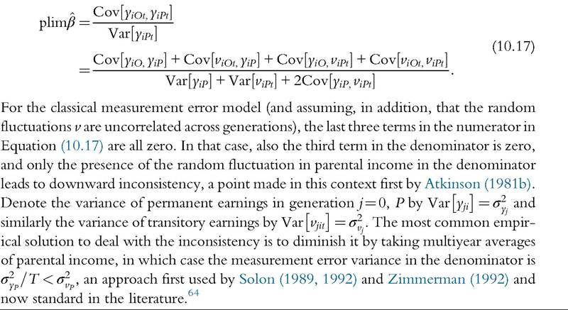
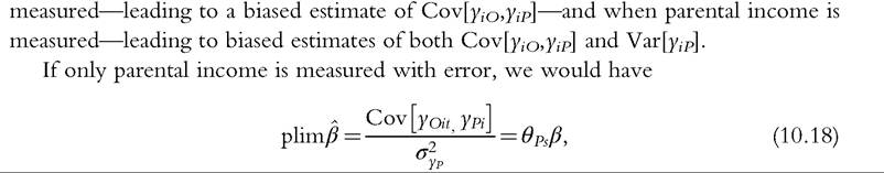 where s is the age at which parental income is measured, and
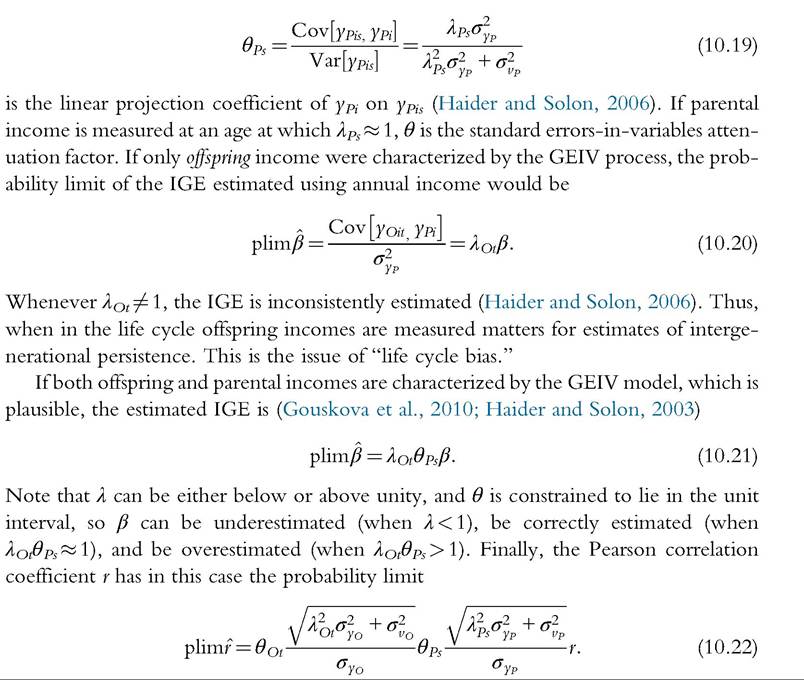
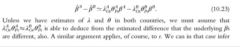
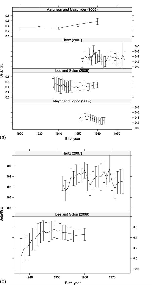

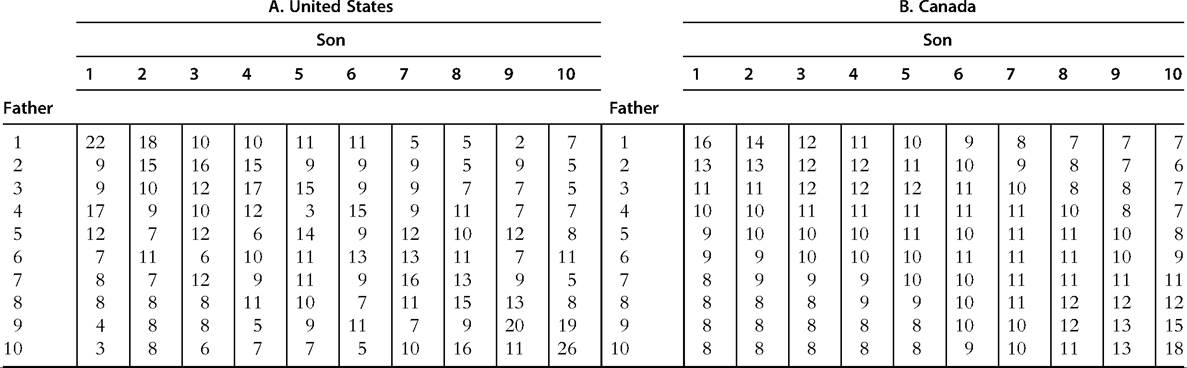
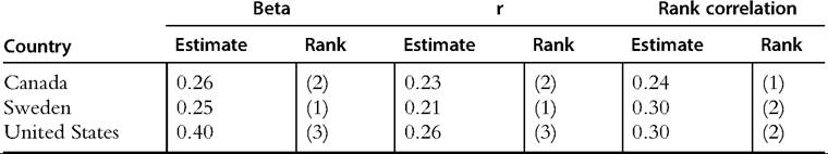
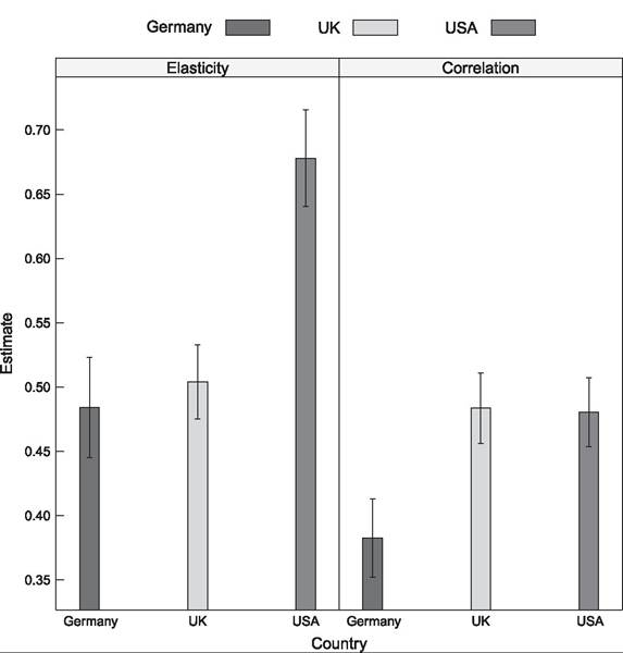
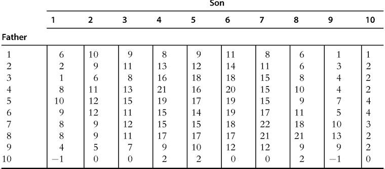
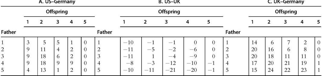

 The share of the variance of long-run income that can be attributed to
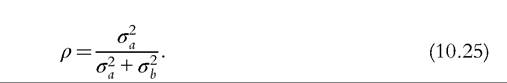
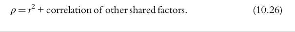
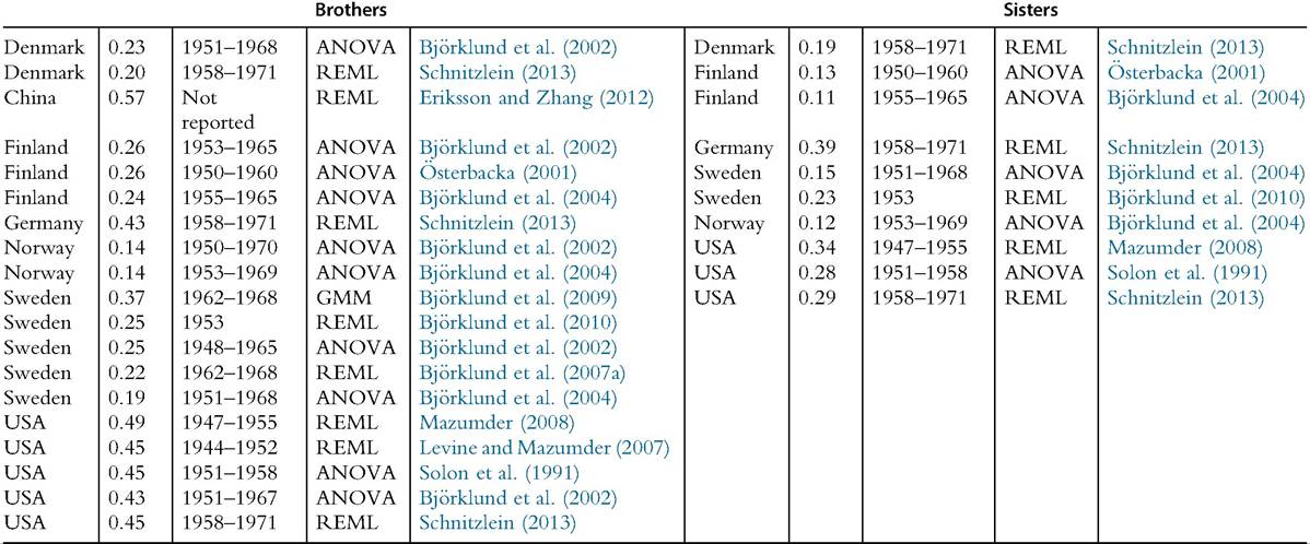
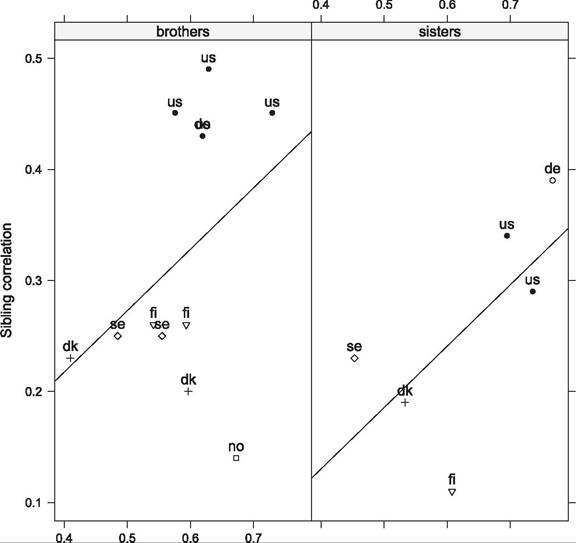
More on the topic Intergenerational mobility: evidence:
- Atkinson Anthony, Bourguignon François. Handbook of Income Distribution. Volume 2A. North Holland,2014. — 2366 p., 2014
- PREPARING THE GROUND FOR EMPIRICAL ANALYSIS