MOBILITY MEASUREMENT

This section is about measuring mobility. First we discuss descriptive devices, by which we mean graphical and tabular methods for summarizing patterns of mobility. We con­sider them in more detail than other surveys because we think it is important to “let the data speak” (though there are limits to which this is possible, as we show).

10.3.1 Describing Mobility

In the two-period case, the bivariate joint distribution of income contains all the infor­mation there is about mobility, so a natural way to begin is by summarizing the joint distribution in tabular or graphical form.^[582] How one proceeds depends on the nature of the data to hand and the mobility concept of interest. We have been assuming that income distributions are continuous but in practice it is often convenient to represent the data in grouped form, or the data may be intrinsically discrete as in the case of “social classes.” In addition the information content of the descriptive device is related to the way (if any) in which the analyst standardizes the marginal distributions of any one bivariate distribution and, when making comparisons of bivariate distributions, makes further adjustments (e.g., to control for differences in average income between the bivar­iate distributions for two countries). If one is solely interested in pure exchange mobility (changes in relative position), then both issues are dealt with by working with the frac­tional rank implied by an individual’s income rather than the income itself.

A mobility matrix, M, is constructed by first dividing the income range of each mar­ginal distribution into a number of categories (which need not be the same in each period, but typically is) and cross-tabulating the relative frequencies of observations with each matrix cell: typical element m_i j is the relative frequency of observations with period 1 income in range (group) i and period-2 income in range j. The graphical representation of the discrete joint probability density function is the bivariate histogram. Alternatively, the mobility process may be represented by the transition matrix and the marginal distributions. Borrowing notation from Atkinson (1981a), suppose that there are n income ranges, with the relative number of observations in group k in period-1 is m#8542; for k = 1,..., n, and correspondingly in period 2. The marginal (discrete) distribution in period-1 is summarized by the vector m₁ = (m1, m2,..., m1) and correspondingly for period-2. Hence,

m^k₁ = m^k2A. (10.2)

When the focus is on pure exchange mobility, the ranges typically refer to quantile groups. For example, in the case of decile groups, each group contains one-tenth of the population. The transition matrix is then bistochastic. Mobility is entirely character­ized by the transition matrix A.

An illustrative example is shown in Table 10.1. Mobility refers to changes in the rel­ative positions in the United States between 1979 and 1988, and 1989 and 1998, with each individual’s income defined as the equivalized real annual family disposable income of the family to which the individual belongs. The United States in the 1980s and the 1990s is a long way from the total immobility scenario (in which every cell percentage would equal to zero, except those on the leading diagonal, which would equal 100%).

If the interest is in mobility other than of the positional kind, changes in the marginal distributions are also of interest. A particular example might be when the income class boundaries are defined as fractions of median income, or as fractions of the poverty line and there is interest in poverty rate trends as well as movements into and out of low

Tah#8739;P 1#8745; 1 Dpriln tr#964;#953;n#962;iti#8745;n m3trirp#962;- Ilnitprl Rtatp#962; #915;#964;#8745; 1Q7Q— 1 QRR ëïã³ ÃÌ 1QRQ-1QQR ÃïðããðïÒëïðñ³

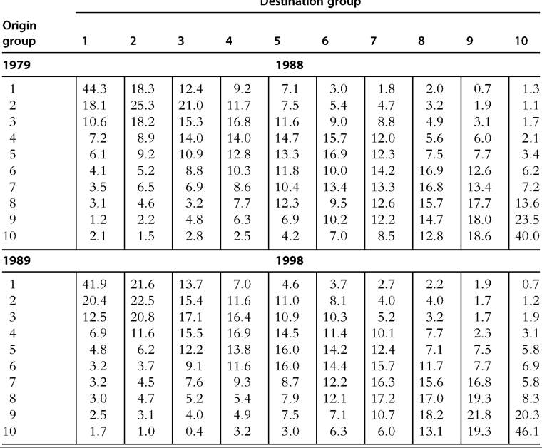
Note: Income refers to equivalized real annual family disposable income, distributed among all individuals (adults and chil­dren). The decile groups are ordered from poorest (1) to richest (10).

Source: Hungerford (2011, Tables 2 and 3), based on PSID data.

income.^[584] More generally, defining income group boundaries that are fixed in real income terms over time provides indications about individual income growth for indi­viduals of different origins; if each period’s incomes are standardized by period-average income, the information refers to income growth relative to the average.^[585] (We say “indications” regarding this mobility concept because its essence refers to income changes at the individual rather than group level.) Similarly, the dispersion across origin groups of individuals from a common income origin may be indicative of income risk, but the connection is not altogether obvious. Neither mobility matrices of this kind nor conventional transition matrices are directly informative about mobility as longer-term inequality reduction.

Graphical summaries can complement and sometimes be more effective than tabular presentations; visual impact matters. Even transition matrices and comparisons of them can be visualised. We refer, for instance, to the use of transition probability color plots introduced by Van Kerm (2011). Suppose individuals are classified into vingtile groups in each of period 1 and period 2. For the visualization, individuals are classified according to their income group in period 2, and lined up in rows with the poorest twentieth in one row at the top, the next twentieth in the row beneath, and so on down to the final row containing the richest twentieth. Each person is also tagged with their period-1 group membership using a color coding system. Suppose the poorest twentieth in period 1 is represented by blue and the richest twentieth by red, and the intermediate groups are represented by the colors of the rainbow in between. If there were no changes in relative position over time, every one would remain in their period-1 income group; there would be a one-to-one correspondence between rows and colors.

Examples of such representations, due to Van Kerm (2011), are shown in Figure 10.1 for individuals’ household income mobility between 1987 and 1995 in Western Germany (left) and the United States (right). It is immediately apparent that, over this 12-year period, there is substantial income mobility in both countries and throughout the income distribution, including a small fraction of the richest twentieth falling to

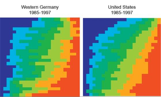
Figure 10.1 Transition color plot examples. Source: Van Kerm (2011). (For color version of this figure, the reader is referred to the online version of this book).

the poorest twentieth, and vice versa. But there is clearly no origin independence in either country, let alone complete rank reversal. Interestingly, however, it is also clear that the main differences in patterns of mobility are at the bottom of the income distri­bution (more changes in relative position in Western Germany than in the United States). We return to this finding in the next section. The particular advantage of the transition color plots is their visual immediacy. However, color is not always available. The color transition plots summarizing income mobility in the book by Jenkins (2011a, Figure 5.1) were reproduced in black and white, and this reduced their effectiveness.

What about alternative devices? Perhaps the most straightforward way to summarize a bivariate joint distribution is using a scatter plot of period-2 incomes against period-1 incomes. Figure 10.2 provides a within-generation example using British income data for 1991 and 1992.

The advantages of the scatter plot are that it is very easy to produce and provides an immediate impression about the degree of immobility of incomes (the clustering around the 45° line), as well as the nature of the marginal distributions. For a focus on changes in relative position alone, the corresponding scatter plot would be of individuals’

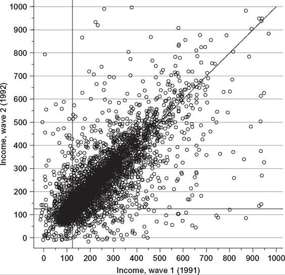
Figure 10.2 Scatter plot example. Source: Jenkins (2011a, Figure 1.2).

normalized ranks in each of the two periods. The main disadvantage is that potentially important detail is lost because the bivariate density is not estimated; there is no difference to the eye between 10 observations with a particular combination of period-1 and period-2 incomes and 100 observations with the same pair of incomes.

One way to proceed is derive and plot the joint density. The simplest estimates to produce are those of the bivariate discrete density (essentially plotting the bivariate histogram—see above). However, there are well-known disadvantages of such discreti­zation: As in the univariate distribution case, the estimates are sensitive to choice of income class boundaries, and of course, information within the ranges is lost with the grouping. Kernel density estimation methods avoid the problem because of the way in which they smooth data within a moving window rather than within fixed categories. Figure 10.3 shows a “typical” joint bivariate density for West German family incomes for 2 consecutive years over the period 1983—1989.^[586] Incomes in each year are normalized by the contemporaneous median, but otherwise, the marginal distributions are not con­strained to be the same (so this is a representation of exchange mobility alone). Compared to the scatter plot, the concentration of individuals on and around the 45° representing perfect immobility is readily apparent. However, the fine detail remains difficult to

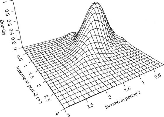
Figure 10.3 Bivariate density plot example. Note: The charts shows a “typical” kernel density estimate for incomes in two consecutive periods. Source: Schluter (1998, Figure 1).

14

ascertain, partly because the three-dimensional representation has to use a specific pro­jection. What a reader perceives may change if the estimates are viewed from a different angle. Related, differences in marginal distributions are difficult to examine; so too is individual income growth. A further issue, shared with the scatter plot and bivariate his­togram, is that it is difficult to compare a pair ofbivariate distributions (e.g., for two dif­ferent countries), even if the plots to be compared are placed adjacent to other. Overlaying one plot on another is far too messy, but without some form of overlay, detailed comparisons are constrained.

Both issues are resolved to some extent by summarizing the density estimates using contour plots in which contour lines connect income pairs with the same density. An example is provided using U.S. and West German income data for 1984 and 1993 in Figure 10.4. Income refers to the log of equivalized family income expressed as a devi­ation from the national contemporaneous mean. Contour lines are drawn at values that separate the quintile groups for each country (the 20th, 40th, 60th, and 80th percentiles). The solid lines are for the United States, the dotted lines are for West Germany (WG).

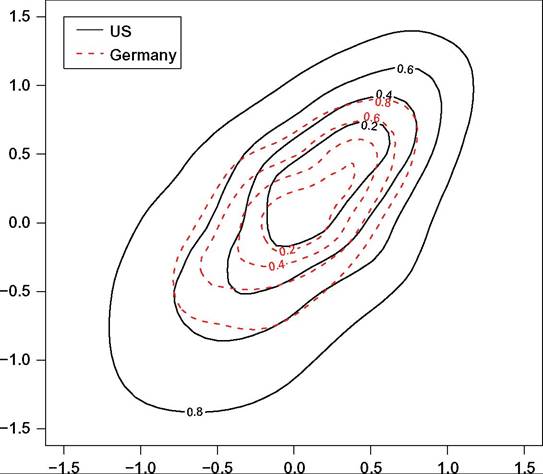
Figure 10.4 Contour plot example. Note: The chart shows the kernel-smoothed joint density of income in 1984 and 1993 for the United States and West Germany, where income is posttax posttransfer family income equivalized by the PSID equivalence scale, and income for each year is expressed as a deviation from the year-specific mean. Source: Gottschalk and Spolaore (2002, Figure 1), redrawn by the authors.

As Gottschalk and Spolaore (2002) commented, the plot reveals multiple features of the joint distribution. Each contour line for Germany lies inside its U.S. counterpart, indi­cating greater cross-sectional inequality in the United States. Clustering around the 45° immobility line is apparent for both countries but is greater for the United States. Also, the contour lines are generally flatter for Germany, meaning that expected period-2 income (conditional on period-1 income) varies less with period 1 in WG than it does in the United States. Gottschalk and Spolaore (2002) commented that this suggests a lower cross-period correlation in the United States, and they also pointed to a greater variation around the conditional means in the United States. Contour plots are also used in the U.S.-West German comparisons by Schluter and Van de gaer (2011, Figure 2).

Just as contour plots for continuous income distributions correspond to mobility matrices, there are also devices for continuous incomes corresponding to the transition matrix. One requires estimates of the conditional density f(y#8739;x), which is straightfor­wardly estimated in principle using the fact that f(y#8739;x) =f(y,x)#8725;f(x). Estimates of the numerator and denominator are derived across a grid of values of x and y using kernel density estimation. See Quah (1996), who refers to this concept as a “stochastic kernel” and applications to income mobility include Schluter and Van de gaer (2011). Compared to unconditional joint density plots, the conditional density plots allow a more direct comparison of expected income growth across the base year income range. Examples are provided in Figure 10.5 based on data for the United States (top chart) and Western Germany (bottom chart) for 1987 and 1988. Income is equivalized net household income expressed relative to the 1987 median. Schluter and Van de gaer (2011, p. 11) pointed to not only the greater spread of contours in the United States indicating differences in mar­ginal distributions, but also that the “particular... feature of the conditional densities is the greater upward mobility of low-income Germans” compared to low-income Americans. Note the more distinct upturn of the contours in the top left of the Western German chart compared to the shape of the corresponding U.S. contours.

Conditional densities are not the same as conditional probabilities, which is what constitute the transition matrix. Estimation of the conditional (cumulative) probability density F(y#8739;x) requires integration over the marginal distribution of y. As Trede (1998) explained, estimates of F(y #8739;x) can be inverted to give the probabilities for second-period income conditional on particular values of first-period income (“p-quantiles”). Trede’s device for “making mobility visible” is a plot of these p-quantiles against first-period income values. Figure 10.6 shows one of these nonparametric transition probability plots using data for West German equivalized family incomes in 1984 and 1985. Incomes are normalized by the 1984 median, so “growth mobility is not excluded from the analysis” (Trede, 1998, p. 80). In the extreme case of origin independence, each transition proba­bility contour would be horizontal. If, instead, there were complete immobility so that second period incomes were completely determined by first period incomes, the contours would lie on top of each other. (In particular, if there were no change in median income,

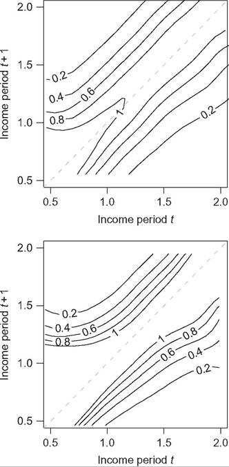
Figure 10.5 Conditional density plot example. Note: Year t refers to 1987; year t+ 1 refers to 1988. The top chart refers to the United States; the bottom chart to Western Germany. Source: Schluter and Van de gaer (2011, Figure 2).

the contours would lie on the 45° line.) The greater the gaps between the contour lines, the greater is inequality in the second period. The slope of the contours is generally less than 45°, indicating some regression to the median. Figure 10.6 shows that, among individuals with median income in 1984, around 10% have an income less than 0.7, and about 10% have an income of at least 1.7 of the 1984 median in 1985. Methods closely related to Trede’s are used by Buchinsky and Hunt (1999) to derive nonparametric esti­mates of transition probability estimates, which the authors reported in tabular rather than chart form.

Patterns of mobility in the form of individual income growth are not shown directly in the devices discussed so far. The simplest way to focus on this aspect is to define income

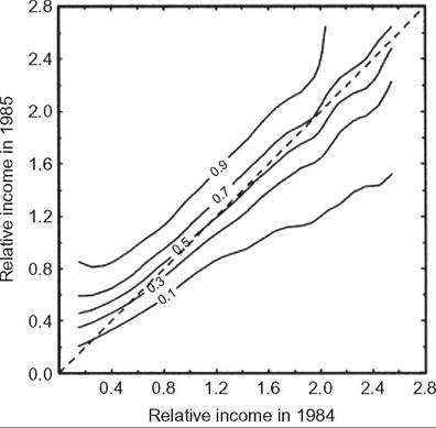
Figure 10.6 Nonparametric transition probability plot example. Note: Relative income in each year equal to income divided by the 1984 median income. Source: Trede (1998, Figure 1).

growth at the individual level between the two periods using some measure of directional income growth (Fields and Ok, 1999b), thereby converting the bivariate joint distribu­tion to a univariate distribution of income changes. Then all the devices commonly used for summarizing univariate income distributions are available with one important proviso. Income changes may be negative or zero and not restricted to positive values (and the mean change may also be zero or negative). However, the ratio of second- period income to first-period income is positive (assuming incomes are positive), and it is often convenient to use this metric. Schluter and Van de gaer (2011, Figure 2) present kernel density estimates of the distribution of income ratios. Comparisons based on plots of cumulative distribution functions (CDFs) of income change distri­butions are also presented by Chen (2009, Figure 4) and Demuynck and Van de gaer (2012, Figure 1).

A CDF plot of this type is based on an ordering of individuals’ income changes from smallest (most negative) to the largest. One is often interested in the extent to which individual income growth is “pro-poor,” that is, whether income growth is greater for those at the bottom of the first-period income distribution relative to those at the top. In particular, pro-poor growth between two periods is a factor reducing the the inequality of second period incomes relative to first period incomes.^[587] See also the dis­cussion of SWFs in Section 10.2. Fields et al. (2003) plotted the average change in log per capita income between two time points against income in the base year, for four countries. Comparisons across countries are constrained by the fact that the income range on the horizontal axis (base-year income) varies tremendously. Comparability is enhanced if, instead, one plots individuals’ average income change against their nor­malized (fractional) rank in the base-year distribution (with individuals ordered from poorest to richest). The horizontal axes in this case are bounded by 0 and 1. Such plots were developed by Van Kerm (2006, 2009) and independently by Grimm (2007). Extensive empirical examples are provided by Jenkins and van Kerm (2011) for four 5-year periods in Britain during the 1990s and 2000s, from which Figure 10.7 is taken. (Individual income growth refers to the change in the log of individuals’ household income between 2 years.) It is clear that income growth is distinctly pro-poor in each of the subperiods, especially 1998-2002.^[588]

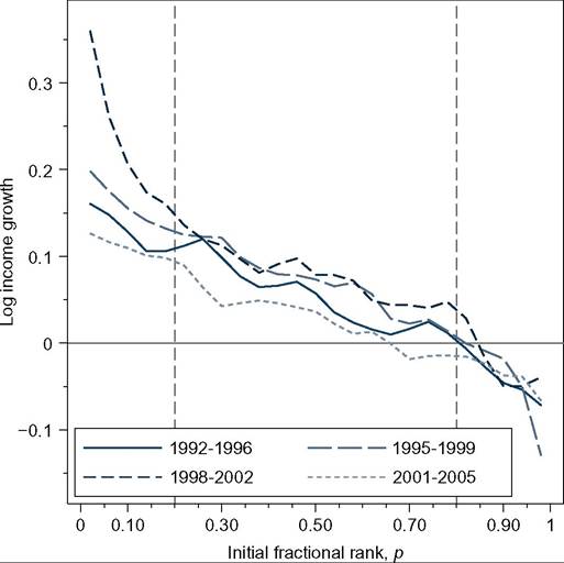
Figure 10.7 Individual income growth and mobility profiles. Source: Jenkins and Van Kerm (2011).

In sum, we have reviewed a portfolio of tabular and graphical devices for summarizing income mobility between two periods. By standardizing marginal distributions in differ­ent ways, different aspects of the mobility process can be focused on, and for individual income growth, there are separate devices.

Within-generation income mobility analysis has tended to use graphical summaries and comparisons rather more than between-generation mobility analysis, which has mainly relied on transition matrix tabulations for detailed summaries of the mobility pro­cess. In part, this emphasis is because the mobility concept most associated with interge- nerational mobility is pure positional change totally separate from any changes in the marginal distributions. Nonetheless, there do appear to be opportunities forgone to use other methods to describe the distribution.

Our final observation here is that there appear to be no straightforward descriptive summaries that directly highlight the concepts of mobility as longer-term inequality reduction or as income risk. We consider the former case later. In the latter case, one wants something analogous to the mobility profile but, instead, of summarizing expected (average) income growth conditional on base-year income or income position, one would summarize conditional income dispersion.

10.3.2 Mobility Dominance

Dominance checks are a widely used part of the analyst’s toolbox for comparing univar­iate distributions of income. To what extent can and should this be the case for mobility comparisons? We identify three main approaches.

The most well-known dominance results are those of Atkinson and Bourguignon (1982). The results are derived with reference to the social welfare framework discussed earlier. Social welfare is the expected value of individuals’ utility-of-income functions defined over period-1 and period-2 income, where individual utility is a concave trans­formation of the per-period utilities of income and also increasing in each income.

Welfare comparisons of differences in mobility for bivariate distributions f andf* are based the difference

where #916;f(x, y) =f-f* is the difference in bivariate densities and the same U(.) is used for the social evaluation of each distribution (cf.Equation 10.3).

Analysis has focused on the case in which the marginal distributions x and y are iden­tical, and SWFs satisfy the conditions U₁ gt; 0, U₂ gt; 0, and U₁₂ lt; 0 (guaranteed if U(x,y) is a concave transformation of the sum of the per-period utilities). Atkinson and Bourguignon (1982) showed that a necessary and sufficient condition for a welfare improvement #916; W#8805; 0 is that #8710;F(x,y) #8804; 0 for all x and y. That is, differences in the cumulative bivariate distribution are lower at each point (a first-order stochastic dominance condition).

What sorts of differences between joint distributions are associated with such condi­tions being satisfied? Atkinson and Bourguignon (1982) discussed the case of a “correlation-reducing transformation,” which leaves the marginal distributions unchanged but reduces the correlation between x and y:

When the bivariate distribution is represented using a transition matrix, this transforma­tion is equivalent to shifting probability mass away from the matrix diagonal.^[589] The cumulative density can be straightforwardly derived by cumulation across cells of the transition matrix starting from the lowest origin and destination group. For comparisons of two transition matrices, first-order welfare dominance exists when the difference in cumulative densities in corresponding cells is everywhere of the same sign. Atkinson (1981a,b) demonstrates the approach in action using intergenerational income data for Britain. Further examples are provided later in this chapter.

The dominance result is a notable addition to the toolbox for comparisons of bivariate distributions but, perhaps surprisingly, has not been widely used. There are several rea­sons for this. The first is that, although relevant to evaluations of pure positional change mobility, the Atkinson-Bourguignon SWF is primarily sensitive to mobility as reversals rather than mobility as origin dependence (see the earlier discussion).^[590]

Second, the first-order dominance checks have not provided clear cut rankings in practice (cf Atkinson, 1981a,b). A natural reaction in this case is to seek unanimous mobility rankings according to more restricted classes of SWFs using second- and higher-order dominance checks. Atkinson and Bourguignon (1982) provide the theo­retical results. The problem, however, is that the additional restrictions on the SWF are hard to interpret. They involve the signs of third- and fourth-order partial derivatives of U(x,y). Although Atkinson and Bourguignon pointed out that in the case of homo- thetic preferences, “the signs of higher derivatives depend on the relation between the degree of “inequality aversion”... and the degree of substitution” between periods (Atkinson and Bourguignon, 1982, p. 18), i.e., the relation between parameters #949; and #961; discussed earlier, they do not elaborate. It is difficult to understand what the sign condi­tions mean in everyday language.

Third, analysts may be interested in alternative concepts of mobility besides positional change. Individual income growth is the most prominent example of this situation. As

discussed earlier, researchers have used social evaluation functions that are increasing functions of a measure of “distance” between first and second period incomes for each individual i, d(x_i,y_i) and defined social welfare as the socially weighted sum over individ­uals of the d_i. For instance, Fields et al. (2002) undertook checks based on comparisons of pairs of CDFs of d_i, where d_i is defined in six different ways in their empirical application. However, as remarked earlier, their SWF has unappealing properties. The challenges involved in the derivation of stochastic dominance results for Fields and Ok (1999b) type measures of nondirectional income movement are discussed by Mitra and Ok (1998). Van Kerm (2006, 2009) explicitly derived dominance results for two classes of SWF defined over the d_i. The first is when the social weights are simply assumed to be positive. Van Kerm showed that unanimous rankings by this evaluation function are equivalent to nonintersections of mobility profiles (the graphical device discussed earlier), a first-order dominance result. If one also assumes that the social weights are nonincreasing functions of base-year income ranks (poorer individuals receive higher weights), unanimous social welfare rankings are equivalent to nonintersections of cumulative mobility profiles. Bourguignon (2011) showed that dominance conditions can be derived for SWFs more closely related to Atkinson and Bourguignon (1982) ones, but the conditions are difficult to interpret intuitively and, in any case, are restricted to the case in which marginal dis­tributions in the initial year are identical.

Dardanoni (1993) derived stochastic dominance results for rankings of mobility pro­cesses that are summarized by transition matrices, focusing on pairs of monotone matrices with the same steady-state income distribution.^[591] The SWF is defined on a vector con­taining each individual’s lifetime expected utility (the discounted sum ofper-period util­ity values, where each income class has a common utility value associated with it; there is no within-class inequality in utility). Overall social welfare is not the average of the indi­vidual lifetime expected utilities because linearity combined with anonymity would imply that mobility is irrelevant for social welfare assessments (as discussed earlier). Instead, Dardanoni’s SWF is “a weighted sum of the expected welfares of the individuals, with greater weights to the individuals who start with a lower position in the society” (Dardanoni, 1993, p. 371). Thus there is a direct parallel with the social weight system employed in the welfare function used by Van Kerm (2006, 2009).

Dardanoni shows that unanimous social welfare rankings by this evaluation function can be checked by comparisons of the cumulative sums of the “lifetime exchange” matri­ces corresponding to the two transition matrices. (A lifetime exchange matrix summarizes the joint probability that an individual starting in some income class i is in lifetime income class j.) These matrices depend on the discount factor underlying them: Although in gen­eral mobility processes that improve the position of initially poorer individuals are more highly valued, the timing of utility receipt also matters. Dardanoni (1993) provided addi­tional results for checking the robustness of dominance results to the choice of discount factor. The fact that actual societies may not be in steady state and transition matrices may imply different steady-state distributions limits the applicability of the dominance results. Dardanoni (1993) acknowledged this, but also pointed out that this could be remedied by focusing on bistochastic quantile transition matrices (as Atkinson, 1981a,b) did, in which case attention is restricted to changes in relative position). The orderings derived differ from those of Atkinson (1981a,b), however, because the SWF is different. For instance, Dardanoni (1993) pointed out that maximal mobility according to his ordering corre­sponds to the situation of origin independence, not rank reversal. Finally, we observe that Dardanonfs dominance results appear to have been rarely used. As with the results of Atkinson and Bourguignon (1982), we suspect that is because applied researchers have found them relatively complicated to interpret and implement.

In sum, we have shown that there are dominance results for mobility comparisons, but the “toolbox” is much less settled than it is for comparisons of univariate income distributions. In part, the reason comes back (again) to the fact that there is a multiplicity of mobility concepts and (related) a lack of consensus about how to specify the SWF function in the bivariate case.

10.3.3 Mobility Indices

In this section, we review indices that might be used to summarize intra- and interge- nerational income mobility. After a brief discussion of generic properties of indices, we discuss some commonly used measures of bivariate association—what Atkinson et al. (1992) refer to as “intuitive” measures—and then move on to more specialist indices (i.e., ones more directly corresponding to the various mobility concepts identified ear­lier). Whether an index focuses on positional change, individual income growth, longer- term inequality reduction, or income risk accounts for many of its properties. There are general features on which we contrast indices.^[592]

First, there are different normalizations. Although all indices equal zero in the case in which there is complete immobility, there is no shared maximum mobility value and, indeed, some measures have no maximum value imposed (principally the indices of income growth and income risk). Second, there is a distinction between “pure” measures of positional change and other indices. The former indices, of exchange mobility, are sensitive only to the (re)ordering of individuals and hence with values unaffected by any monotonic transformation of each income between time periods (or, equivalently, also unaffected by changes in the marginal distributions of income). By contrast, struc­tural measures register mobility even if ranks are constant but the income values associ­ated with those positions change over time.

20

Third, and related, indices differ in how they reflect income changes that are common to all persons, whether by the same proportion or by the same absolute amount. Measures are “strongly relative” (“intertemporally scale invariant”) if equiproportionate income growth does not affect the mobility assessment. Measures are “weakly relative” (or “scale invariant”) if the units in which income are measured are irrelevant but, by contrast with strongly relative measures, equiproportionate income growth may count as mobility.^[593] There are also translation invariance counterparts of these properties. Again, the principal distinction is between measures of pure positional change (exchange mobility)—which satisfy both intertemporal translation and scale invariance—and the other indices. For example, most indices of longer-term inequality reduction are scale invariant but not intertemporal scale invariant. Most indices of individual income growth are neither intertemporal scale nor translation invariant.

Fourth, there is the issue of directionality, which refers to the roles played by the base year and current year in mobility assessments. An index is directional if it matters whether a particular income change refers to a change from a base year to a current year or vice versa. This is relevant if one wishes to take the temporal ordering of changes into account, and this is particularly important for measures of individual income growth, as one would want to treat differently an income change from 100 to 150 and an income change from 150 to 100. One would want the former to represent an improvement in circumstances, and the latter a deterioration.

Fifth, indices may satisfy various decomposability properties. Mobility indices may be (additively) decomposable by population subgroup, as inequality indices are, according to which total mobility can be written as the weighted sum of mobility within subgroups defined by an exhaustive nonoverlapping partition of the population in question accord­ing to some characteristic (e.g., sex, age, or education) plus (possibly) a term representing between-group mobility. Most indices of longer-term inequality reduction can be decomposed, thus and so too can individuals of income growth, though there is typically no between-group mobility term in that case.^[594] Measures based on changes in ranks are not decomposable because in general there is no one-to-one correspondence between an individual’s rank in his/her subgroup and in the population as a whole.

A second type of decomposability is into structural and exchange components. Unlike decompositions by population subgroup, these decompositions are not additive and rely for their derivation on the use of Counterfactual income distributions represent­ing the situations when there is an absence of exchange mobility or of structural mobility. On this, see, e.g., Markandya (1984), Ruiz-Castillo (2004), and especially Van Kerm (2004).

A third decomposition idea, most commonly exploited in measures of individual income growth or income flux refers to intertemporal consistency—whether mobility calculated for income changes between times t and t + s is the sum of the mobility between times t and t + r and between t + r and t + s (with r lt; s) or, alternatively, the prod­uct. This is the concept of additive (alternatively, multiplicative) path separability or path independence. A fourth mobility-related decomposition relates changes between two years in inequality measured by the change in a generalized Gini coefficient to the sum of two mobility indices—one of progressive income individual income growth and the other of reranking. SeeJenkins and Van Kerm (2006) for details.

We refer to these features at several points in what follows. We now turn to consider the most commonly used “statistical” or “intuitive” measures of (im)mobility, which are the Pearson (product moment) correlation, r, between the log of incomes at two time points or its close sibling Beta (#946;), the slope coefficient from a least-squares linear regres­sion of log(period-2 income) on log(period-1 income):

#963;₁

r = #946; ¹, (10.4)

#963;₂

where #963;₁ and #963;₂ are the standard deviations of log incomes in periods 1 and 2. Put dif­ferently, r is #946; scaled by the changes in inequality in the marginal distributions as assessed by the variance-of-logs inequality index, and it measures the degree of regression to the (geometric) mean in income between periods 1 and 2. H = 1 — r is the Hart (1976) index of mobility, the properties of which are discussed in detail by Shorrocks (1993) and often used in the intergenerational mobility context. H ranges between — 1 and 1, and H = O in the case of complete immobility.

Beta, as we shall discuss later, has been used in almost every empirical study of inter­generational income mobility (1 — #946; is an index of mobility). This is perhaps surprising because it is the positional mobility concept that has been of the greatest interest in this context, and yet Beta and r (or H) reflect structural as well exchange mobility. A perfect linear relationship between period-2 and period-1 incomes (r = 1, H = 0) is consistent with unchanged ranks but also income growth. It is sometimes argued (see Section 10.5) that r is more suitable than Beta as a measure of income (im)mobility when undertaking cross-national comparisons on the grounds that r controls for differences in marginal dis­tributions. But such controlling is only done to a rather limited extent, because changes in inequality are only one distributional feature (and uses one particular inequality measure to do so). Differences in marginal distributions would be fully controlled, however, were analysts to employ the Spearman rank correlation rather than r (because both marginal distributions would be standard uniform distributions), and this would also have the advantage in the intergenerational context of focusing on positional change. Note also D’Agostino and Dardanoni (2009a) who provided an axiomatic characterization of the Spearman rank correlation as an measure of exchange mobility, thereby taking it beyond being a mere “statistical” index.

A second question regarding Beta and r is why they should be calculated using log incomes rather than incomes. To be sure, Beta is a unit-free measure (an elasticity), but this begs the question of whether we are interested in immobility as the lack of a linear or log-linear relationship.^[595]

All in all, there are probably two reasons for the continuing widespread use of Beta and rin the intergenerational mobility literature. The first, as we discuss in Section 10.5, is that various methods to assess the impact of measurement error, and discussions of the relationship between Beta, r, and sibling correlations, rely on properties of regression and moments. The second reason is simply inertia: researchers continue to use Beta because they want to compare their estimates with those of others before them. The main problem with Beta as a measure that intergenerational mobility researchers have noted is its scalar nature rather than more fundamental concerns about the mobility concepts that are reflected in it. Their developments of “vector” measures take us some back toward the more detailed graphical summaries of bivariate distributions discussed earlier.

For example, instead of fitting a single log-log regression, researchers have estimated quantile regressions of period-2 incomes on period-1 incomes (see, e.g., Eide and Showalter, 1999). (The periods refer to offspring and parental generations, rather than years within a generation.) However, it is not immediately clear what the estimates tell us about (im)mobility. At a technical level, the answer is clear. A quantile regression of, say, the 10th percentile of son’s income on father’s income allows the researcher to express the 10th percentile of son’s income as a function of father’s income. The quantile regression coefficient on father’s log income then measures the elasticity of the particular quantile of son’s income with respect to father’s income. Differences in estimates across the quantiles tell us how sensitive different parts of the son’s distribution conditional on father’s income are to small changes in father’s income. However, why these marginal changes, measured by slopes of the conditional quantiles, are of interest is not obvious.

One way to interpret the information provided by the vector of quantile regression coefficients is in terms of the full conditional distribution of son’s income. Apicture that is familiar to most students of regression analysis is the fitted regression line from a regres­sion with one explanatory variable, with the distribution of the error term around that line drawn in a few different levels of the explanatory variable. In the classical case, all those distributions are the same, or at least have the same variance (i.e., the error term is homoscedastic). If the distribution of y₂ (for sons), conditional on y₁ (for fathers), is homoscedastic, all estimated quantiles would have the same slope coefficient (save for random error). If the regression slopes are greater for higher percentiles of the son’s dis­tribution, it suggests that the conditional variance of son’s income may be increasing with father’s income.

23

Comparisons of the quantile regression estimates with the Beta from the loglinear regression can also reveal some further aspects of the distribution of period-2 incomes conditional on period-1 incomes. The log-linear regression line gives the conditional expectation, and the regression slope for the 50th percentile gives the expected median. Ifwe find that for most of the range of father’s incomes that the conditional mean for sons is lower than that of the relevant father’s income, this suggests that, conditional on father’s income, son’s income is skewed to the left, rather than skewed to the right (as is usually true for income distributions). One can also use the predicted percentiles for different values of father’s income to generate summary distributional statistics for the conditional distribution. For instance, one can derive the (discrete) CDFs for period-2 (son’s) income, conditional on a set of period-1 (father’s) income percentiles. One could then check, e.g., whether the distributions first-order stochastically dominate each other. (This relates to Monotonicity assumption of Benabou and Ok, 2000.) Any conditional summary statistics can be generated this way, including inequality statistics such as per­centile ratios. Individual income growth summaries such as in Figure 10.7 refer to con­ditional expectations (means) of distributions like these (except that they are typically drawn at different base-year ranks rather than different base-year income levels). In sum, there are close connections between some of the “vector” measures of mobility and the graphical devices discussed earlier. In what follows, we return to focusing on sca­lar measures.

The second most common type of intuitive measure is an “immobility ratio” (IR). IRs summarize how much clustering there is on (or, sometimes, also around) the leading diagonal of a transition matrix—and hence summarize positional change. For example, for a decile transition matrix, an IR might be defined as the percentage of all persons who remain in the same decile group between the two periods. (A variant would be to cal­culate the percentage remaining in the same decile group or on either side of it.) Clearly, the IR equals 100% in the complete immobility scenario. If, instead, there is complete independence of origin, the IR for a decile transition matrix is 20% (52% in the variant). An index of mobility can easily be calculated as 1 — IR.

Shorrocks (1978b) proposed a mobility index closely related to the IR, a Normalized Trace measure, equal to [n — trace(A)]#8725;(n — 1), where A is the transition matrix with n income classes and trace(A) is the sum of the transition proportions on the leading diagonal of A. This provides a neatly normalized index: with complete immobility, trace(A) = n and the normalized trace equals 0; with complete origin independence trace(A) = 1, and so the normalized trace equals 1.

By construction, an IR and the Normalized Trace are insensitive to any differences between transition matrices aside from those in the respective diagonals. Bartholomew’s (1973) AverageJump index is a positional mobility measure that addresses this aspect. It is equal to the number of income class boundaries crossed by an individual (whether upward or downward), averaged over all individuals (and equal to 0 in the complete immobility case). One feature of the AverageJump index is that it generalizes to the sit­uation when the researcher has individual-level data on incomes rather than simply grouped data (a transition matrix). The index is then the population average of the abso­lute changes in fractional ranks (i.e., the ranks normalized to range from 0 to 1 rather than from 0 to the population size).

The transition matrix also offers, as a by-product, measures of low and high income persistence defined in terms of rank-order immobility. Mobility matrices, in which class boundaries are defined in real income terms, also do so. For example, if the lowest class boundary in each period is the poverty line, then the mobility matrix shows the propor­tion of individuals who are poor in a base period who are still poor in some later period (or who escape poverty). And with repeated longitudinal data for multiple periods, it is straightforward to define “survival probabilities”—the chances that a person remaining poor for #964; years, where #964; = 1,2,.... One can also define measures of high income per­sistence analogously (and we report some estimates in the next section).

This way of thinking about low-income persistence provides a link with the more well-known literature on poverty persistence, especially the approach pioneered by Bane and Ellwood (1986) in which consecutive periods spent poor are aggregated into spells (summarizing the total time spent poor). Rather than looking at spells of poverty (or affluence), one may simply count the number of times each person is poor (or rich) over some fixed time horizon and summarize that distribution. Low-income persistence sta­tistics of this nature are published by, e.g., the UK Department for Work and Pensions (Department for Work and Pensions, 2009) and the Statistical Office of the European Communities (Eurostat).

There is also a nascent literature developing indices of poverty persistence that focuses attention on the way in which people’s experience of poverty over time is aggregated, and hence how to compare, say, a history of 3 consecutive years in poverty followed by 3 years of nonpoverty, with a history in which the person was poor every second year in the six-year period. Research in this topic can be found in Foster (2009), Gradin et al. (2012), Mendola et al. (2011), Mendola and Busetta (2012), and Porter and Quinn (2012). This literature works with a time horizon of fixed length and summarizes indi­viduals’ experiences within that window, ignoring whether poverty spells were already in progress at the beginning of the window or remained in progress at the end of the win­dow. If one wants to derive the shape of the poverty spell distribution in the population (rather than simply the sample), these issues of left- and right-censoring of poverty spell data (which are ubiquitous) need to be accounted for. They are given great attention in the spell-based literature on poverty persistence following Bane and Ellwood (1986), which, on the other hand, ignores longitudinal aggregation issues.

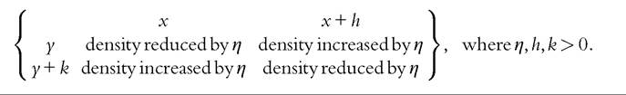
We now turn to a selection of more specialized indices of positional change that have been less commonly used than the ones mentioned so far. The first is the Gini Mobility index of Yitzhaki and Wodon (2005). It is based on the idea of mobility as (lack of) correlation but, instead of using the Pearson or Spearman correlations, it uses the Gini correlation, which, like other Gini-based measures, focuses on ranks rather than income levels per se. The Gini correlation between the income distributions in periods 1 and 2 is

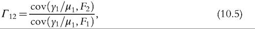
where y₁#8725;#956;₁ is period-1 relative income (i.e., income divided by the period-specific mean income), F₁ and F₂ are the fractional ranks in the two periods, and cov(.) means covariance. Because 1 — #915;₁₂ is a directional measure of mobility (#915;₁₂ = #915;₂₁ in general), the overall Gini mobility index is defined as a weighted average of the two possible direc­tional measures, where the weights depend on the inequalities in each marginal distribu­tion, measured using the Gini coefficient (G). That is,

Yitzhaki and Wodon (2005) showed that if there is no positional change, the Gini mobil­ity index equals 0, it equals 1 if there is complete origin independence, and it equals 2 if there is complete rank reversal.^[596]

The Gini mobility index uses a particular weighting function when aggregating changes in individuals’ ranks but one that is not immediately clear. By contrast, the King (1983) index takes an explicit welfarist approach in which differences in social weights across ranks are defined and tuned parametrically. The basic building block is the “scaled order statistic” for each individual i, s_i, equal to the absolute magnitude of the difference between i’s period-2 income and the period-2 income that i would have had, were she/he to have maintained the same rank in period 1, all expressed relative to mean period-2 income. There is complete immobility if s_i = 0 for all individuals. Using an approach analogous to that of Atkinson (1970), King defines his mobility index as the proportion of total period-2 income that society would be prepared to forego to have the mobility observed rather than complete immobility (positional change is socially valued). Assuming a homothetic form for the SWF leads to a mobility index depending on two parameters—the degree of aversion to period-2 income inequality and the degree of aversion to income immobility (larger values of which give greater social weight to mobility, other things being equal). For generalizations of and commentary on King’s approach, see Chakravarty (1984) and Jenkins (1994).

24

On the one hand, the systematic welfarist approach used by the King index (and others like it) has much to recommend it. On the other hand, it relies on a rather special characterization of what counts as mobility at the individual level (the scaled order sta­tistic), in which the implications for social welfare of changes in ranks are summarized by income values and a particular no-mobility thought experiment. Also the SWF does not depend directly on incomes in period 1, except insofar as they characterize s_i. Compare this with the Atkinson and Bourguignon (1982) SWF defined over incomes in periods 1 and 2 that was discussed earlier. Gottschalk and Spolaore (2002) embraced (and extended) the latter in the first part of their article, but when they later defined specific mobility indices, they use an approach that is similar to King’s (1983) in that the social gains from mobility are all expressed relative to a complete immobility reference point, and this is defined in the same way as in the King index. To develop their indices, Gottschalk and Spolaore (2002) also assumed homotheticity in their SWF, and the resulting class has three parameters, representing aversion to multiperiod inequality, rank reversal, and origin dependence. Although each parameter has a clear interpretation when taken individually, thinking about the implications of different combinations of values is more complicated. We are aware of no use of the Gottschalk and Spolaore (2002) indices other than by the authors themselves.

We move now to consider measures of individual income growth. As mentioned in the Introduction, these incorporate two basic ideas: (i) income increases for an individual count positively in the social calculus and income decreases count negatively, and (ii) total income growth is a function of income growth values for each individual (and the mea­sure of each person’s income growth depends only on their incomes in the two periods, and not the incomes of other people). The first idea refers to the directionality of the income growth measure. The second is a form of decomposability property across indi­viduals, and also leads to aggregate measures that are decomposable by population sub­groups. Although the empirical applications of these measures have all been to intragenerational income mobility, the indices could also be applied to intergenerational income mobility when there is interest in structural mobility over and above exchange mobility.

Fields and Ok (1999b) provided the most well-known aggregate measure of direc­tional income growth in this tradition.^[597] They show that directional measures ofindi- vidual income growth that satisfy the properties of scale invariance, subgroup decomposability, and multiplicative path separability must take the form

25

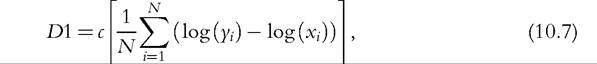
where c is a normalizing constant, which may be set equal to one, and N is the population size. That is, overall income growth is the average of individuals’ proportional income growth. This is the case in which (directional) distance between incomes, d(x_i,y_i) = log(y_i) — log(x_i). Observe that the social weighting scheme treats all individuals the same, regardless of their base-year income and regardless of how much income growth each experiences. Both these aspects, and some other generalizations, have been incorporated in later work.

Demuynck and Van de gaer (2012) used axioms similar to Fields and Ok (1999b), but explored the implications of assuming additive as well as multiplicative path separability, and also of imposing an axiom of “priority for lower growth” that builds in aversion toward inequality in the individual growth rates. The axiom states that “aggregate growth increases more when additional income growth is allocated to individuals with lower income growth than when it is allocated to individuals with higher income growth” (Demuynck and Van de gaer, 2012, p. 750). The authors prove that the measure satis­fying their axioms is of the form:

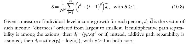
When #948; = 1, the general indices reduce, in the first case, to the directional measure of Schluter and Van de gaer (2011) and, in the second case, to the Fields and Ok (1999b) measure described earlier (with #960; = c, and also normalized to 1). In Schluter and Van de gaer’s (2011) index, #960; is a sensitivity parameter, with higher values increasing the “distance” measured between incomes in period-1 and period-2 but keeping ranks the same. Demuynck and Van de gaer (2012, p. 754) remarked that when #948; = 1, correlation-reducing transformations to incomes in either period of the kind discussed earlier increase mobility according to S but D1 is insensitive to such changes. In the more general case, with #948; gt; 1, more weight is given to individuals with smaller values of d,#8729;. When #948; = 2, the weights are like the weights used to characterize the Gini coefficient of inequality and when #948; #8594; #8734;, only the smallest d_i counts. In these more general cases, S is no longer additively decomposable by population subgroup, and it is possible for correlation-decreasing transformations to reduce mobility. The larger question, how­ever, concerns the social desirability of “priority for lower growth”: why should we be concerned about the inequality of individual growth rates (the d,#8729;) independently of incomes in the initial or final period? Because of this issue, and (related) the greater com­plexities involved with using a two-parameter index, we conjecture that empirical researchers will be more likely to use S with #948; = 1 than the more general case.

The directional measures of income growth of Jenkins and van Kerm (2011) are built using a different approach and relate to a SWF defined as the weighted average of the d_i (see Section 10.2), in which the social weights are a decreasing function of period-1 income ranks, defined using a single-parameter generalized Gini scheme.²⁶ Put differ­ently, Jenkins and van Kerm (2011) build in a social preference for pro-poor income growth, and the choice of different parameter values provides indices ranging from lim­iting cases in which aggregate growth is the simple average of the d_i values (as with D1) or in which only the growth rate for the poorest period in the initial year counts.²⁷ Palmisano and Van de gaer (2013) provide an axiomatic characterization of the Jenkins and van Kerm (2011) class of measures. The usefulness of these indices rests largely on the extent to which the concept of pro-poor income is viewed as a desirable normative prin­ciple: see the discussion in Section 10.2 about the link between progressive income growth and inequality reduction.

The pioneering paper on mobility as reduction in the inequality of longer-term income is by Shorrocks (1978a). The essential insight is that, were one to longitudinally average each person’s income over a number of years (T, say), the inequality in these averaged incomes would be less than average annual inequality because each individual’s income fluctuations would be smoothed out and no longer contribute to aggregate cross­sectional dispersion in incomes for the T-year accounting period. Shorrocks (1978a) defined a measure of income rigidity, R(T), equal to the ratio of inequality among T-averaged incomes (“longer-term” inequality) to the weighted average of single-year 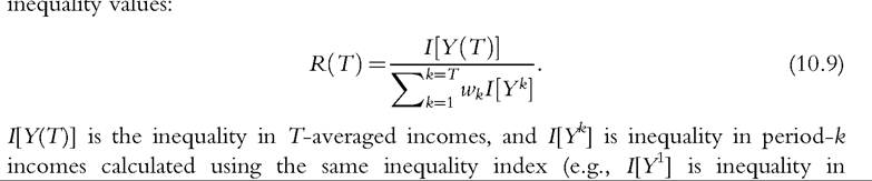period-1 incomes). The weights w#8539; are the proportion of aggregate T-averaged income received in period k (i.e., w_k=#956;_k#8725;#956;), and the weights sum to unity. Shorrocks shows that if one restricts attention to conventional relative inequality indices, then R is bounded

above by 1. When there is complete rigidity in relative incomes, inequality in each period corresponds to inequality for the longer accounting period.^[598] The more frequent or larger that income changes are, the less rigid the income system, and thus one may define a measure of mobility: M(T) = 1 — R(T).

As Shorrocks (1978a, p. 178) puts it, “mobility is regarded as the degree to which equalization occurs as the observation period is extended.” In terms of the properties dis­cussed earlier, M(T) is a nondirectional index and scale invariant (because it is defined in terms of relative incomes), but not intertemporal scale invariant (given the way in which the per-period weights are defined). Although R and M are usually used to describe within-generation mobility, in principle they could also be used to describe mobility between generations. R and M are distinctive in that they are well defined when there are data for many periods, but they can also be calculated if there are only two (the typical situation with intergenerational data).

A nice feature of the Shorrocks approach is that it can be used in two ways. The first is to calculate a single index value conditional on a particular value of T (and inequality index). This fixed-window calculation can be employed, e.g., to examine trends in income mobility over time in a country using moving fixed-width windows. Second, one can examine how R(T) changes as T is increased from its minimum value of 1 to some larger maximum (i.e., there is one window, the width of which is varied). The resulting rigidity and mobility profiles provide a straightforward graphical device for comparisons of the extent of mobility within a country, and also comparisons across pop­ulation subgroups and countries. Rigidity profiles for the United States and Western Germany from a pioneering cross-national study of income mobility discussed further in the next section are shown in Figure 10.8. The profile for Western Germany lies everywhere below that for the United States: Whatever the accounting period used, mobility is greater in Western Germany than in the United States.

Clearly, the values derived for the Shorrocks indices are conditional on the inequality index employed for the calculations. It is also well known that inequality indices differ in the sensitivity to income differences in different parts of the income distribution (Atkinson, 1970). So, it is important to know how estimates of rigidity and mobility relate to choice of inequality index, and how differences in inequality index sensitivity translate into mobility index sensitivity. It has been found as an empirical regularity, from Shorrocks (1981) onward, that using different indices can make a big difference to the estimates of R derived and also that the Gini coefficient tends to show greater R values

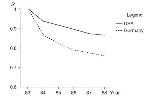
Figure 10.8 Income rigidity (longer-term inequality expressed as a fraction of total inequality) falls as the time period is lengthened. Note: Income is posttax posttransfer income. The Shorrocks rigidity index R is computed using the Theil index of inequality. “Germany” refers to the federal states of Western Germany. Source: Burkhauser and Poupore (1997, Figure 2).

than other inequality indices. The explanation is that “[since] the main effect of cumu­lating income is to average out incomes that are temporarily high or low, the strongest egalitarian trend will be found in the tails. The distribution of relative incomes in the middle range is not substantially affected by cumulating incomes over time” (Shorrocks, 1981, p. 182). Combine this information with the fact that the Gini coeffi­cient is relatively insensitive to income transfers in the tails of the income distribution, and we have the result.

The sensitivity of R to the choice of inequality index is examined more systematically by Schluter and Trede (2003). For the two-period case, they show that the global rigidity measure, R, can be expressed, to a good approximation, as the weighted average of “local” rigidity comparisons at each point along the income range of a value for the longer-term averaged income, and the average of the per-period distributions. Differ­ences in global measures arise, therefore, from a combination of differences in the way the different inequality indices summarize local comparisons at each point along the income range, and the different weighting systems that they incorporate. Schluter and Trede (2003) show that the sensitivity of mobility measure to choice of inequality index is partly dependent on data, but they also show some clear empirical regularities. For example, the weighting functions for commonly used generalized entropy indices and the Gini coefficient are broadly similar around the middle of the distribution (relative income = 1) and tend to place greater weight on mobility at the tails of the distribution. In addition, the overall U-shape for the weighting function is distinctly shallower for the Gini than for the other indices (as Shorrocks argued). Given the ready availability of longitudinal data on incomes nowadays (see the next two sections), it is straightforward for researchers to examine sensitivity empirically.

Refinements to the Shorrocks approach have gone in two main directions. The first addresses the assumption that individuals are able to smooth incomes across time: see the discussion in Section 10.2. This aspect is relaxed by Maasoumi and Zandvakili (1990) and Zandvakili (1992), building on Maasoumi and Zandvakili (1986). See also the survey by Maasoumi (1998). The basic idea is to allow for different degrees of substitutability between incomes in different periods. Thus, rather than defining longer-term income for each individual as the simple arithmetic average, it is defined as a generalized mean for which the choice of a parameter tunes the degree of substitutability. A common parameter is used for each individual, and yet one would expect the ability to smooth income over time to vary with, e.g., income level. Incorporating such heterogeneity into an index would be a rather complicated exercise and has not been done, as far as we are aware. As it is, researchers wishing to implement the Maasooumi-Zandavakili variant on R need to choose a substitutability parameter as well as inequality index. Of course, esti­mates can easily be derived for a number of combinations but the volume of results pro­duced is probably one reason the approach is not commonly used. Also, the empirical illustrations provided by Maasoumi and Zandvakili (1990) and Zandvakili (1992) tend to suggest that the more general index tended to provided qualitatively similar results to that of the Shorrocks approach.^[599]

The second refinement to the Shorrocks approach is to reconsider the reference point against which longer-term inequality values are compared. The main argument of Fields (2010, p. 410) is that “[w]hat we as empirical researchers would want to know in a given context is the extent is the extent to which the mobility that takes place works to equalize longer-term incomes relative to base, disequalizes longer-term incomes relative to base, or has no effect” (emphasis in original). This leads to Fields’ proposal that the denominator in the expression for R be changed from the weighted average of the per-period inequal­ities to the inequality in first-period income. Chakravarty et al. (1985) emphasized rather different aspects in the derivation of their mobility index: they were concerned with “ethical” indices of relative income mobility, which are derived from SWFs and measure changes in welfare. Mobility is the percentage change in social welfare (measured by the equally distributed equivalent income, defined in the Atkinson (1970) sense) of the actual distribution of longitudinally averaged incomes compared to what social welfare would have been in the completely immobile benchmark distribution—taken to be the observed period-1 distribution.

If the same welfare function is used to evaluate both distributions, and that SWF is homothetic, then the mobility measure “has a natural interpretation; it is the percentage change in equality of the aggregate distribution compared with the first-period benchmark” (Chakravarty et al., 1985, p. 6). Although the authors go on to state that it appears there is no convincing ethical argument for applying the same welfare function to both distributions, all empirical applications that we are aware of have applied the same welfare function. The class of mobility indices for the two-period case is then defined as (Chakravarty et al., 1985, p. 8):

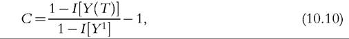
where I is a relative inequality index equal to one minus an index of relative equality (as is the case with the Atkinson (1970) class of inequality indices). It turns out that the Fields (2010) mobility index, 1 — [I[Y(T) = I[Y¹], equals #954;C where #954; = (1 — I[Y(T)]) = I[Y¹], and so the measures are closely related (assuming the same inequality index is applied in each case). But it is possible for them to differ about whether mobility has increased or not: the value of #954; matters. In short, ethical index C always evaluates mobility as welfare-increasing (but of different degrees), whereas the more descriptive Fields (2010) index allows mobility to be positive or negative. A more fundamental issue, com­mon to both indices, is whether one agrees with the proposal to accord special normative status to period-1 incomes relative to incomes in other periods—which is an issue that has arisen with other mobility measures as well.

The concept of comparing short- and longer-term incomes has been used to examine poverty persistence in particular as well as income mobility in general. The basic building block is again “longer-term income,” a measure of longitudinally averaged income for each individual, and people are defined as “chronically” poor if their longer-term income is less than the poverty line. Chronic poverty in aggregate is the poverty in the population calculated using a poverty index that is additively decomposable over people and time (e.g., a member of the Foster et al., 1984 class). Transitory poverty is Total Poverty (poverty calculated over individuals and separate time periods) minus Chronic Poverty. The main papers to date in this tradition are Rodgers and Rodgers (1993, 2009), Chadhuri and Ravallion (1994), and Jalan and Ravallion (1998). See also the development by Duclos et al. (2010), which takes a more explicitly welfarist approach. As with the Shorrocks mobility measures, there is an important issue concern­ing how longer-term incomes are calculated and (related) the assumptions made about abilities to income smooth. See, e.g., the discussion by Rodgers and Rodgers (1993, pp. 34—35).

The final group of more specialist mobility indices we discuss are those that summa­rize notions of income risk. These can be classified in two main ways. On the one hand, there are measures of the transitory variance of (log) income, calculated using either model-based or nonparametric approaches and generally requiring income data for mul­tiple periods. On the other hand, there are measures of income flux, income movement, and volatility, generally defined over incomes in two periods only. We consider the approaches in turn and discuss the relationships between them and the measures of longer-term inequality reduction.

To fix ideas,^[600] [601] suppose that the dynamics of income for each individual can be described using the canonical random effects model

where y_it now refers to the income for person i in year t. It consists of a fixed “permanent” random individual-specific component, u_i, with mean zero and constant variance #963;2 (common to all individuals), and a year-specific idiosyncratic random com­ponent with mean zero and variance #963;2 (common to all individuals) that is uncorrelated with u_i. Thus total inequality as measured by variance of log incomes is equal to the sum of the variance of “permanent” individual differences plus the variance of “transitory” shocks:

Assuming that permanent differences are relatively fixed over time, changes over time in income inequalityarise mostly through changes in the variance of the transitory component. The interpretation of this latter component as idiosyncratic unpredictable income change leads to the association of changes in its variance with changes in income risk.

This canonical model is patently unrealistic in several respects, and three types of extension have been incorporated. The first additional factor allows the relative impor­tance for overall inequality of the permanent and transitory components to change with calendar time. For example, if there is an increase in the demand for skilled labor, and permanent component of income represents relatively fixed personal characteristics related to skills (for example human capitals of various kinds), then greater inequality resulting from widening differences over time in returns to skilled versus unskilled labor can be represented as the growing importance of the permanent component. In contrast, a secular trend toward greater labor market flexibility can be represented as a growth in the importance of transitory variations. The second additional feature is persistence in

transitory shocks. The factors leading to a temporary fall (or rise) in income in one year are likely to have effects that last longer than a year: a transitory shock persists but with diminishing impact and eventually dies out. An example might be an accidental injury leading to a reduction in work hours that diminishes over time. This is usually charac­terized using an autoregressive moving average process for v_it.

The third modification to the canonical model is to allow the fixed individual com­ponent to change over time. Two main approaches have been followed, originally dis­tinct but now commonly combined. One is to allow u_i to vary over time via a “random walk”: this year’s value is equal to last year’s value plus or minus a random element. The second approach allows for individual-specific rates of growth in income (the “random growth” model). The expression for the permanent component is modified so that it also varies linearly with time but with heterogeneity in this slope. Both a random walk and random growth lead to a fanning out of the income distribution over time, other things being equal. Rankings are preserved; those at the bottom stay at the bottom but fall fur­ther behind those at the top, who stay at the top. It is increases in the transitory variance that increase mobility in the sense of reranking.

The estimation of transitory variances (mobility) and permanent variances using these models is common, but has also been criticized on the grounds that estimates are sensitive to the particular model specification employed, and there are potential identification issues with the relatively short household panels used to estimate the models (see, e.g., Doris et al., 2013; Guvenen, 2009; Shin and Solon, 2011). This has led to simpler non­parametric methods also being regularly used.

The most common nonparametric method for deriving estimates of variance com­ponents is the window-averaging method first employed by Gottschalk and Moffitt (1994), also known as their BPEA method (the acronym refers to the journal in which their work was published). The BPEA method works by first calculating the longitudinal average of each person’s log income over a time window of fixed width, say T years. This provides an estimate of the person’s “permanent” income for that period and is directly analogous to the longer-term income concept used to derive R except that it refers to averaging of log incomes. (IfEquation 10.11 describes the income-generation process, the longitudinal average is an estimate of u_i.) The transitory incomes for each individual within the window are derived as a difference between this permanent income and observed log income, from which can be calculated the individual-specific transitory var­iance. The overall sample transitory variance is the average of these variances. The sample permanent variance for each window is calculated from the differences between each person’s permanent income and the sample grand mean of these, with an adjustment to account for the fact that the mean contains a proportion of the transitory component that has not been fully averaged to zero over the T-year window. See Gottschalk and Moffitt (2009, p. 7) for full details of the formula, and Kopczuk et al. (2010, p. 98) for a small variation on the same theme. The BPEA method is known to provide biased estimates of the transitory variance and its trend if the permanent component’s contri­bution changes over time (see, e.g., Shin and Solon, 2011). Using shorter-width win­dows for the calculations (smaller T) reduces the potential impact of this problem, but at the cost of reducing the statistical reliability of the estimate of each person’s permanent income.

It is inevitable that measures derived using methods like the BPEA one will reflect the variability from permanent shocks and not only from transitory shocks. Shin and Solon (2011, p. 977) argued that this is a virtue of such measures: “The recent interest in vol­atility trends stems in large part from a concern about whether earnings risk has increased. Because permanent shocks, such as those experienced by many displaced workers, are even more consequential than transitory ones, it makes good sense to include them in the measurement of earnings volatility.” Their own calculations use instead a measure of volatility that will be discussed shortly.

Both of the two main methods for estimating transitory variances have potential weaknesses, and there are virtues in using both as well as other measures (such as of volatility) as a sensitivity check. (This is increasingly done, as the next section shows.) Regardless of estimation method, there is a distinction between measures of mobility that are based on the transitory variance itself and measures that are based on the transitory (or permanent) variance expressed as a proportion of the total var­iance. Most discussion uses the former as the definition of mobility in the form of income risk.

Some authors also present estimates of the permanent variance expressed as a propor­tion of the permanent variance, and note that, if estimated using the BPEA method, there is a close relationship with the estimates of the Shorrocks measure of income rigid­ity R. See, e.g., Burkhauser and Couch (2009) and also Chen and Couch (2013, p. 202), who state that they prove that “under one testable condition a measure of economic mobility formed by the ratio of permanent to total variance employing the methods of Gottschalk and Moffitt (1994) is equivalent to the Shorrocks R constructed with a Theil General[ized] Entropy Index.” It is clear that there must be some relationship, but we believe that it is not as close as stated by these authors, for the simple reason that the BPEA method calculation uses log incomes, and calculations of R invariably use incomes expressed in levels rather than logs. Evidence showing that a BPEA-estimated ratio of permanent to total variance and Theil-based estimate of R can move in opposite directions appears in Bayaz-Ozturk et al. (2014, Figure 2). For a related discussion, see also Shorrocks (1981, Section 6), who considers the shape of the profile for M(T) in the case in which incomes—not log incomes—follow the basic canonical random effects model (cf.Equation 10.11) and inequality is calculated using half the squared coefficient of variation. He shows that were the model to hold, M(T), would converge to its lim­iting value fairly rapidly. Slow convergence is evidence that the canonical model is inappropriate.

Income volatility in a given year t, V_t, is commonly measured by the standard devi­ation (SD) of the distribution of individual changes in log income between 1 year and an earlier year:^[602]

Changes are typically measured over a one- or two-year horizon: #964; = 1 or 2. The Fields and Ok (1999b) index of individual income growth (D1 discussed earlier) is the mean of the distribution of log-income changes. Volatility is therefore a measure of dispersion of the same distribution using one specific index of inequality. There are further connec­tions: Ifthe Gottschalk-Moffitt BPEA method is used to calculate the transitory variance in the two-period case, the resulting estimate is equal to one-quarter of the variance of the change in earnings (i.e., V_twith T = 2). See Moffitt and Gottschalk (2012, p. 218), who also point out that the relationship no longer holds if the data window is longer than two periods.

This brings us to the measures of income flux, most commonly associated with the names of Fields and Ok (1996, 1999b), who proposed a number of measures ofnondir- ectional income movement for the two-period case. Although such indices are rarely related to the measure of income risk discussed so far, their inventors had this application in mind: “A measure of income movement... identifies how unstable the incomes of individuals have been throughout the time period. Since income instability may cause economic insecurity,... measure of income movement are useful complements to the traditional measures of relative income mobility” (Fields and Ok, 1999b, p. 455). In their 1996 paper, Fields and Ok consider what they label absolute measures of income movement. First, they propose a number of axioms to describe measures for a fixed pop­ulation of N individuals: linear homogeneity (equi-proportionate increases in all incomes, in base and final year, lead to the same proportionate increase in the measure); translation invariance; a normalization axiom; decomposability (total mobility for the N individuals is a symmetric function of the income changes for each individual); growth sensitivity (if two bivariate distributions are identical except that in one distribution an individual experiences more income movement than in the other distribution, total mobility differs in the two distributions); and, finally, the axiom of individualistic con­tribution (the contribution of each individual’s mobility to total mobility does not depend on how other people’s incomes change).

Fields and Ok (1996) prove that the measure satisfying these seven axioms is the sum over the N individuals of the absolute differences between period-1 and period-2 incomes (i.e., #8739;y_i — x,#8729;#8739;, for each individual i = 1,..., N). The final step is to consider versions of these measures that would enable comparisons across populations of different sizes. Specifically, their per capita measure of absolute measure of absolute income move­ment is

Their “percentage” measure is the same as D2 except that the denominator is total income in period 1 rather than population size and has been less commonly used perhaps because it is unclear that the base year should be used as the reference point (see our earlier discussion).

In their 1999 article, Fields and Ok took a similar similar set of axioms but also con­sidered scale-invariant measures of movement as well as translation-invariant ones. This leads to the per-capita relative movement index, given by

Both D2 and D3 are additively decomposable by population subgroup: total income movement can be expressed as the weighted sum of the movement within each sub­group, where the weights are the subgroup population shares. Fields and Ok (1996, 1999b) show that D2 and D3 also satisfy a different sort of decomposition: in each case, aggregate income movement can be expressed as the sum of a component representing income “growth” for individuals and a residual component that can be interpreted as income “transfers” between individuals. (Slightly different versions of the decomposition apply depending on whether the average of the first component is positive or negative.) It turns out in the case of D3 that the growth component of this decomposition is the direc­tional measure of proportionate income growth (D1) discussed earlier.

To return to the remarks earlier about the links between measures of income flux and other measures of income risk, observe that the variance of log-income changes between two periods can be written as E(d_i)² — E²(d_i), where E is the expectation operator, and d_i = log(y#8539;_+#964;) — log(y_it). That is, volatility-squared is equal to the average of the squared log-income changes, minus the square of the average log-income change. The first term is a measure of income flux in which the distance concept used to record income changes is Euclidean distance. Thus, there is a close relationship between orderings by this measure and a volatility measure when average log-income changes are “small.” This Euclidean distance measure is characterized axiomatically by D’Agostino and Dardanoni (2009b), who also compare their approach with that of Fields and Ok (1996, 1999b). A measure incorporating the Euclidean distance concept is also characterized axiomat- ically by another pioneering paper on the measurement of income movement, by Cowell (1985) (see also Cowell and Flachaire, 2011) The axiom set is rather different in Cowell’s

(1985) paper, however, and also leads to parametric classes of subgroup decomposable measures of “distributional change.” These indices have rarely been used in empirical applications, however, perhaps because their properties (in particular the implications of choosing different parameters) are rather opaque in comparison with the overt trans­parency of measures like D2 and D3.

This completes our review of the many measures of income risk. A question that could be asked about all of them is whether they actually measure income “risk” in a more fundamental sense, namely the ex ante uncertainty aspect drawn attention to by, e.g., Gottschalk and Spolaore (2002). As Creedy et al. (2013, p. 236) remind us, this requires a model of expectations formation based on observed income dynamics. There are also additional complications for welfare evaluations such as the extent to which observed income changes reflect voluntary decisions of individual and families and the extent to which these are insurable (and how these aspects differ across people). These complicated underpinnings are absent from the measures we have discussed. At the other extreme are more structural models such as proposed by Blundell et al. (2008) and Cunha et al. (2005). Our overall assessment is that the measures we have discussed are useful descriptive measures despite these flaws. Their relative simplicity facilitates transparency and interpretation as well as empirical implementation. But they should be interpreted cautiously.

Our final remarks concern the applicability of the mobility measures to intragenera- tional and intergenerational data. As we have noted, different mobility concepts may be more relevant in one context than another. For example, positional mobility concerns appear of particular relevance to discussions of intergenerational mobility and income growth of particular relevance to discussions ofintragenerational mobility. But structural intergenerational mobility is also of interest, and so too is the identification of intragen- erational reranking along with income growth. By providing a unified treatment of mobility measures, we hope that some cross-context fertilization may be facilitated. In principle (and data permitting), all the measures we have discussed could be used in either context. In the two sections that follow, reviewing empirical evidence about intra- and intergenerational mobility, we reveal which measures have been used to date.

10.4.