PRELIMINARIES: DIMENSIONS, INDICATORS, AND WEIGHTS

Three questions are preliminary to any discussion of the methods for the multivariate analysis of poverty and inequality: the selection of the relevant dimensions of well-being; the indicators used to measure people’s achievements in these dimensions and the choice of deprivation thresholds in poverty analysis; and the weights assigned to each dimension.

3.2.1 Selection of Dimensions

material living conditions, however, and it may be concerned with “social exclusion.”^[102] According to Burchardt et al. (1999), social exclusion is associated with failures to achieve a reasonable living standard, a degree of security, an activity valued by others, some decision-making power, and the possibility of drawing support from relatives and friends. The variety of dimensions used to define the overall quality of life may be even larger. The Scandinavian approach to welfare, a long-established research program in Nordic countries, considers nine domains of human life: health and access to health care, employment and working conditions, economic resources, education and skills, family and social integration, housing, security of life and property, recreation and culture, and political resources (e.g., Erikson, 1993; Erikson and Uusitalo, 1986-87). Within the “capability approach,” Nussbaum (2003) proposes a specific list of ten “central human capabilities”: life; bodily health; bodily integrity; senses, imagination, and thought; emo­tions; practical reason; affiliation; other species; play; and control over one’s environ­ment.

These examples illustrate the wide range and diversity of the domains considered in the multidimensional analysis of inequality and poverty. The choice of the dimensions that they include is mainly due to the advise of experts, possibly based on existing data, conventions, and statistical techniques.^[103] It could also result from empirical evidence regarding citizen values, or it could be the product of a consultative process involving focus groups and representatives of the civil society or the public at large (Alkire, 2007). In all cases, the selection of poverty and income inequality indicators is a funda­mental exercise, which has to blend theoretical rigor, political salience, empirical mea­surability, and data availability.

In this chapter, we simply assume that a predefined list of r attributes fully describes the well-being concept used in the analysis of poverty and inequality. We ignore all questions concerning the selection of attributes and refer the reader to Chapter 2 for a comprehensive discussion.^[104] Notice, however, that the nature of selected attributes may condition the definition of measurement tools. As noted in the introduction, we cannot mechanically export the Pigou-Dalton principle of transfers, which is central in income inequality analysis to other well-being dimensions, such as health (Bleichrodt and van Doorslaer, 2006), happiness (Kalmijn and Veenhoven, 2005), and literacy (Denny, 2002). Leaving aside the practical problem of how to transfer one unit of health from one person to another, we might doubt that imposing the principle of transfers in the health domain is ethically justified.

3.2.2 Indicators

The indicators used to measure people’s achievements in the various dimensions are numerous and understandably have different measurement units. (Incomes, wealth, and quantities consumed or purchased are continuous variables, but the number of dura­ble goods owned and the frequency in the use of consumer services are discrete variables. Education can be measured by a categorical variable such as the highest school attainment ofa person. Transforming it into the minimum number of years necessary to achieve each school level then provides an objective way to grade the various levels, but we might wonder whether a person who completed 14 years of school is really twice as well- educated as a person who only completed 7 years; moreover, only in a loose sense, can this type of transformed variable be interpreted as truly continuous. People’s com­petencies and problem-solving capacity are increasingly assessed by complex exercises that produce literacy, numeracy, or skill scores generally normalized on a (scale from 0 to 500. These scores are bounded, continuous, ordinal variables.^[105] Individual health and physical status are measured with a host of indicators. Self-reported measures of health conditions are ordinal variables, but the information on the incidence of specific chronic illnesses is dichotomous; anthropometric indicators such as height, weight, and the body mass index are continuous variables. Subjective measures of well-being are typ­ically collected by asking interviewees their personal degree of satisfaction on prefixed numerical scales or verbal rating scales often ranging from “not very happy” to “very happy.” In either case, the outcome is an ordinal variable, which ranks the alternative ratings without however providing any information on how much one rating is better, or worse, than another rating.

Cardinal continuous variables, such as income, probably represent a minority of avail­able indicators of well-being.

Many variables are dichotomous, or binary, either by definition or after a comparison of individual achievement with some social norm: for instance, we may classify those deprived in housing conditions as all individuals living in households with less than one room per person, transforming the variable “room per person” into a binary one. The use of dichotomous variables is at the center of the counting approach examined below.

In poverty assessments, the choice of the indicators is intertwined with the definition of the respective deprivation thresholds. This problem parallels the problem for income or consumption in univariate analysis, with absolute, relative, subjective, and legal criteria being the main alternatives (e.g., Callan and Nolan, 1991). In multivariate analyses, these problems may be amplified by the consideration of intangible dimensions for which it is more contentious to identify minimum thresholds (Thorbecke, 2007). Similar to the uni­variate case, however, the binary distinction between a “bad state” and a “good state” may be too sharp because deprivation might occur by degrees.

3.2.3 Weighting of Dimensions

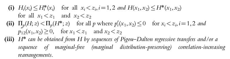
Weights determine the extent to which the selected attributes contribute to well-being and the degree by which we can substitute one attribute for another, interacting with the functional form used to aggregate dimensions. This can be easily seen by defining indi­vidual well-being Sβ as the weighted mean of order β of the achievements in the r dimen­sions, as suggested, for instance, by Maasoumi (1986),

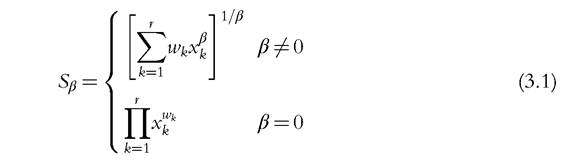
where x_k is nonnegative and represents the level of attribute k, k = 1,2,..., r, and w_k is the corresponding weight. Notice that expression (3.1) turns into an index of deprivation if the r attributes measure hardship. The weights w_k and the parameter β jointly govern the degree of substitution between any pair of cardinal attributes. Indeed, the marginal rate of substitution between attributes b and a, which is the quantity of b that has to be given up in exchange for one more unit of a in order to leave well-being unchanged, is equal to:

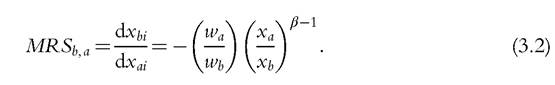
If β = 1 well-being is simply the (weighted) arithmetic mean of the achievements in all dimensions, which are then perfectly substitutable at a rate equal to the ratio of their

respective weights.

The pattern of substitution among attributes can be more muddled than in (3.2) when the functional form of the well-being aggregator is more complex than (3.1), but it is bound to depend critically on weights, except in the extreme cases in which the attributes are perfect complements. The choice of weights might have a significant effect on the results of multidimensional analyses of inequality and poverty. For instance, Decancq et al. (2013) find that the identification of the worst-off in a sample of Flemish people is considerably influenced by the use of alternative weighting schemes of the attributes. In a comparison of the incidence of income-and-health pov­erty in selected European countries from 2000 to 2001, Brandolini (2009) finds that the ranking of Italy and Germany reverses as weights are shifted from one dimension to the other, although the ordering of France and the United Kingdom mostly remains unchanged. Here, we outline approaches to weighting by drawing on Brandolini and D’Alessio (1998), and we refer to Decancq and Lugo (2013) for a more compre­hensive discussion.

A popular way of setting weights is to treat all attributes equally. This is the case with the Human Development Index, which assigns the same weight (one-third) to the three basic dimensions considered: a long and healthy life, access to knowledge, and a decent standard of living (e.g., UNDP, 2013). Equal weighting may result from either an “agnostic” attitude and a wish to reduce interference to a minimum or from the lack of information about some kind of “consensus” view. For instance, Mayer and Jencks (1989, p. 96) opt for equal weighting, after remarking that “ideally, we would have liked to weight [the] ten hardships according to their relative importance in the eyes of legis­lators and the general public, but we have no reliable basis for doing this.” (In fact, there may be disagreement among the legislators and the public, let alone within the public itself.)

Some departure from equal weighting is envisaged by ιAtkinson et al. (2002) and Marlier and Atkinson (2010). They propose a set of principles for the design of social indicators for policy purposes, among which is the principle that the weights should be “proportionate,” so that dimensions have “degrees ofimportance that, while not nec­essarily exactly equal, are not grossly different” (Marlier and Atkinson, 2010, p. 289). This criterion only sets some reasonable boundaries, without specifying how to define unequal weights.

The social evaluator can directly elicit the weighting structure from consultations with groups of experts or the public at large or from the importance assigned to dimen­sions of well-being by survey respondents, or the evaluator can indirectly generate the structure from estimates of happiness equations.^[109] The last procedure is followed by Decancq et al. (2014) who characterize axiomatically a class of multidimensional poverty indices that are consistent with individual preferences in the aggregation of the different dimensions. In addition to standard axioms, they postulate principles for interpersonal poverty comparisons that lead to measuring individual poverty as a function of the frac­tion of the poverty line vector to which the agent is indifferent. The poverty threshold is therefore defined in terms of well-being using person-specific weights. In some exercises, users of statistics are allowed to build their own sets of weights. For instance, the OECD Better Life Index allows people to compare well-being across countries by means of eleven indicators of quality of life that can be rated equally or according to individual preferences (see Boarini and Mira D’Ercole, 2013 and the initiative’s website http:// www.oecdbetterlifeindex.org/). In all these cases, the choice of weights relies on some implicit or explicit normative criterion.

Under certain hypotheses, market prices provide weights that capture a trade-off between dimensions that is consistent with consumer welfare. Sugden (1993) and Srinivasan (1994) contend that the availability of such an “operational metric for weight­ing commodities” makes traditional real-income comparison superior in practice to Sen’s capability approach. Ravallion (2011a, p. 243) argues that the main multidimensional poverty indices aggregate deprivations in a manner that “essentially ignores all implica­tions for welfare measurement of consumer choice in a market economy. While those implications need not be decisive in welfare measurement, it is clearly worrying if the implicit tradeoff between any two market goods built into a poverty measure differs markedly from the tradeoff facing someone at the poverty line.” On the other hand, mar­ket prices may be distorted by market imperfections and externalities, and they do not exist for many constituents of well-being and their imputation may be arduous, although various approaches estimate the “willingness to pay” in order to add the monetary value of nonincome dimensions to income (e.g. Becker et al., 2005; Fleurbaey and Gaulier, 2009; see Chapter 2). More importantly, they may be conceptually inappropriate for wel­fare comparisons, a task for which they are not devised (Foster and Sen, 1997; Thorbecke, 2007).

The main alternative and widely applied approach is “to let the data speak for themselves.” Methods differ, but we may cluster them into two main categories: frequency-based approaches and multivariate statistical techniques. Since Desai and Shah (1988) and Cerioli and Zani (1990), many researchers assume that the (smaller the proportion of people with a certain deprivation, the higher the weight that should be assigned to that deprivation, on the grounds that a hardship shared by few is more important than one shared by many. This approach raises two problems. First, it may lead to a questionably unbalanced structure of weights. As observed by Brandolini and D’Alessio (1998), in 1995, the shares of Italians with low achievement in health and edu­cation were 19.5% and 8.6%, respectively. With these proportions, education insuffi­ciency would be valued more than health insufficiency: one-tenth more according to Desai and Shah’s formula, and over one-half more according to Cerioli and Zani’s for­mula. Whether education should attain a weight so much higher than health is certainly a matter of disagreement. This criterion also makes the weights endogenous to the distri­butions being studied. Thus, it implies that we should take country-specific weights in an international comparison of multidimensional poverty, unless we impose a common, but arbitrary, set of weights. This observation also applies to the suggestions by Betti et al. (2008), who suggest taking weights proportional to the dispersion of the attributes in the population (adjusted for their bilateral correlations to avoid redundancy), and by Velez and Robles (2008), who select weights that allow a set of multidimensional poverty measures to better track the dynamics of self-perceived well-being.

13

Several multivariate statistical techniques are employed to aggregate dimensions.^[110] Maasoumi and Nickelsburg (1988), Klasen (2000), and Lelli (2005) use the analysis of prin­cipal components, on the grounds that this approach.. uncovers empirically the com­monalities between the individual components and bases the weights of these on the strength of the empirical relation between the deprivation measure and the individual capabilities” (Klasen, 2000, p. 39, fn. 13). Schokkaert and Van Ootegem (1990), Nolan and Whelan (1996a,b), and Whelan et al. (2001) use factor analysis to aggregate elementary indicators into measures of well-being or deprivation. These papers tend to use this tech­nique to identify few distinct constituents of well-being, however: as noted by Schokkaert and Van Ootegem (1990, p. 439-40), their application of factor analysis is “a mere data reduction technique,” which does not provide any indication about the relative valuation of each attribute. Several authors apply latent variable models or structural equation model­ing to collapse multiple indicators into indices of total or domain-specific deprivation (Ayala et al., 2011; Di Tommaso, 2007; Krishnakumar, 2008; Krishnakumar and Ballon, 2008; Krishnakumar and Nagar, 2008; Kuklys, 2005; Navarro and Ayala, 2008; Perez-Mayo, 2005, 2007; Tomlinson et al., 2008; Wagle, 2005, 2008a,b). Dewilde (2004) uses a two-step latent class analysis, evaluating deprivation in specific domains in the first step and the latent concept of overall poverty in the second step. Lovell et al. (1994), Deutsch and Silber (2005), Ramos and Silber (2005), Anderson et al. (2008), Ramos (2008, andJurado and Perez-Mayo (2012) apply methods developed in efficiency analysis to aggregate the various attributes of well-being. These methods allow estimating the level of individual achievement relative to the achievement frontier, providing implicit estimates of the values of the weights. In a related approach, Cherchye et al. (2004) con­struct a synthetic indicator to assess European countries’ performance in achieving social inclusion, with weights being variable in order to provide the most favorable evaluation for each country. They contend that this approach preserves the “legitimate diversity” of countries in pursuing their own policy objectives, because a relatively better perfor­mance in a particular dimension is seen as revealing a policy priority.

The methods reviewed in the next sections generally allow for the possibility that weights can differ across dimensions in the social evaluation of poverty and inequality. Our brief overview suggests some ways to define them. Two comments are in order. First, (multivariate statistical techniques differ from other approaches in that their aim is to estimate the level of individual achievement; weights are integral part of the aggre­gation procedure and have no truly independent meaning. We may then wonder whether it is appropriate to use them in conjunction with many of the methods discussed below. Second, as the weighting structure captures the importance assigned to each attri­bute, it is bound to reflect different views. On one side, this suggests questioning the use of techniques that may be robust from a statistical viewpoint but ignore the intrinsically normative aspect of the choice of weights. On the other side, it hints that one way to account for this plurality of views is to specify ranges of weights rather than a single set of weights, although this approach might lead to a partial ordering, as suggested by Sen (1987, p. 30; see also Foster and Sen, 1997, p. 205).^[111]

2.3. MULTIDIMENSIONAL POVERTY MEASUREMENT characteristic makes this “composite index” approach easily understandable and very popular, especially in public debates in which there is a need to summarize headline mes­sages from sets of indicators. If the dimensions of well-being are independent of each other, the order of aggregation does not matter, and the two approaches are equivalent. However, if they are dependent and suffering from multiple deprivations has a more than proportionate effect on people’s well-being, ignoring the impact of the association among the achievements in the various dimensions, as with the composite index approach, may imply overlooking an important aspect of hardship. This is not the case for an indicator such as severe material deprivation in the Europe 2020 strategy, because it would rank a society with one person suffering from four deprivations and three persons not suffering from any differently from a society in which four people fail in one dimension each.

15

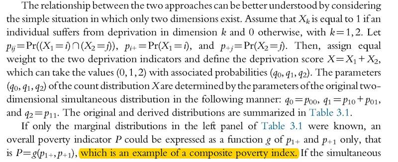
distribution was known, we could turn to the distribution of X in the right panel of Table 3.1, and the overall index could account for the number of deprivations that each in­dividual suffers from. (Counting deprivations highlights two possible ways of identifying someone as poor: either he fails in either single dimension (X = 1), or he fails in both (X = 2). In the first case, we adopt the union criterion: the poor are those with at least one deprivation and P=_ιg(1 — p₀₀). In the second case, we favor the intersection criterion: the poor are those with two failures and P=,g(p₁₁). The contrast between union and

Table 3.1 The distribution Ofdeprivations in two dimensions and the derived distribution of deprivations scores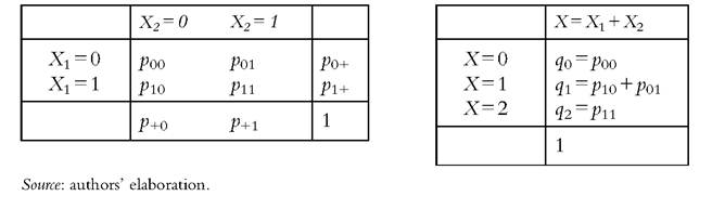

intersection criteria plays a fundamental role in the measurement of multidimensional dep­rivation (see Atkinson, 2003). It also suggests that the occurrence of deprivation in some domains need not entail a condition of overall poverty: if we adopt the intersection crite­rion, only those with two failures are regarded as poor individuals, whereas those with only one failure are not. Setting a critical number of dimensionsto identify the pov­

erty status introduces an additional threshold over those already set for defining deprivation in each dimension (see Alkire and Foster, 2011a,b). We return to this issue in Section 3.3.2.6.

The available information may be richer than the knowledge about the deprived/not deprived status in a number of dimensions, however. Rather than dichotomous, variables may be continuous or discrete with at least three categories. We may then want the overall poverty indicator to account not only for the occurrence of deprivation, that is, an indi­vidual achievement below the given dimension-specific threshold, but also for its intensity, that is, the shortfall of this achievement as compared to the threshold.

These observations illustrate that the reach of the informational basis conditions the multidimensional methods that can be used to measure poverty. When individual-level data on multiple attributes are not available, a composite index may be the only measure that can be calculated. When these data exist but are not publicly available, multidimensional pov­erty analysis may still be possible by using counting measures, if statistical offices release simple tabulations such as those discussed in the examples in Section 3.3.2. We use the com­plexity of informational needs as the criterion to organize the discussion of this section. We begin with the composite multidimensional poverty indices that only require information on the marginal distributions and can be estimated by gathering data from separate sources. All other multidimensional measures need an integrated database in which the information for each relevant dimension is available for each individual unit. We first consider counting measures that use minimal information: the distribution of the population by number of deprivations. With r dimensions, it is sufficient to know r values (the proportions of the population suffering from deprivation in 0,1,..., r dimensions). Although it is the oldest multidimensional approach in social sciences, the counting approach is arguably the least structured from a theoretical point of view, and we devote relatively more space to its exam­ination. Due to its simplicity, the counting approach offers transparent illustrations of alter­native aggregation methods, as well as the role of various normative rearrangement principles, and it helps to clarify the distinction between deprivation and poverty. Next, we turn to multidimensional poverty indices requiring the knowledge of individual achievements in each dimension. Lastly, we discuss criteria for partial ordering.

3.3.1 The Composite Index Approach

We can measure the overall poverty of a society by aggregating over the proportions of individuals suffering from deprivation in the r dimensions of well-being, whenever this is the only available information. A prominent example of this composite index approach is

the Human Poverty Index (HPI), which was published by the United Nations Develop­ment Program from 1997 to 2009 (UNDP, 1997). As originally formalized by Anand and Sen (1997), a general version ofthe index with r dimensions, weighted by w⅛, is defined by 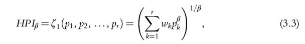where pk is the proportion suffering from deprivation in dimension k (in the two­dimensional case of Table 3.1 p₁ = p₁₊ and p₂ = p₊₁), β > 0, and w_k > 0 for all k; if the r dimensions are equally weighted, w_k = 1/r. As β rises, greater weight is given to the dimension in which there is the most deprivation. UNDP (1997) paid particular attention to three dimensions related to longevity, knowledge, and a decent standard of living, and it later added a fourth dimension, social exclusion, for rich countries. In either case, β was set equal to 3 to give “additional but not overwhelming weight to areas of more acute deprivation” (UNDP, 2005, p. 342).¹6

Bossert et al. (2013) provide an axiomatic characterization of (3.3) for the case in which β = 1, based on the condition of additive decomposability in attributes as well as in individuals (see also Pattanaik et al., 2011). This case is of some interest: it assumes perfect substitutability among the components, and the index HPI₁ equals the weighted arithmetic mean ofthe headcount indices across all dimensions. This implies that people who suffer from k deprivations, with 0 ≤ k ≤ r, are counted k times by the index HPI₁. Although rather crude and ad hoc, this is a simple way of giving heavier weight to people suffering from multiple deprivations. The implicit assumption is that the effect of dep­rivations is proportionate, however: suffering from two deprivations is twice as bad as suffering from one. If there are reasons to question this assumption, then the inability of HPI-type measures to discriminate between situations in which deprivations are con­centrated on few people and situations where an identical total amount of deprivations is spread across many people represents a serious shortcoming.

Dutta et al. (2003) prove that composite indices can lead to the same conclusions as those that would be derived from aggregating first across dimensions and then across indi­viduals only under very restrictive conditions on the aggregation functions. Namely, “the overall deprivation of an individual must be a weighted average of her deprivations [i.e., proportionate shortfalls relative to benchmark values] in terms of the different attributes, and society’s overall deprivation must be a simple average ofthe overall deprivation levels of the different individuals in the society” (Dutta et al., 2003, p. 202). Both conditions may be debatable: the first because it implies that marginal rates of substitution between any pair of attributes are insensitive to the depths of deprivations; the second because it is liable to the same criticism leveled against the poverty gap by Sen (1976). Analogous

16

Chakravarty and Majumder (2005) characterize a general family of deprivation indices that includes an index ordinally equivalent to HPI as a member.

results hold when the equivalence condition is set with respect to rankings rather than indices. Pattanaik et al. (2011) discuss Iurtherweaknesses of HPI-type measures.

Although composite indices may not be consistent with an approach that sees society’s overall poverty as a function of individual poverty levels, as happens in standard welfare economics, they might be justified by taking a different set of ethical assumptions.

3.3.2 The Counting Approach

In many cases, we know more than the headcount poverty ratio for each dimension, and we observe how many people are suffering from deprivation in one dimension, two dimensions, and so forth. Counting the number of failures is well rooted in the analysis of deprivation in social sciences, but the characteristics of the underlying social judgments and the relationship with standard welfare approaches still need clarification. Atkinson (2003), for instance, draws a parallel between the difficulty of deriving dominance con­ditions in the counting case and the failure of the headcount poverty measure to satisfy the Pigou-Dalton principle of transfers in the one-dimensional case. However, this difficulty stems from defining welfare criteria in terms of the distributions of the underlying con­tinuous variables across people rather than in terms of the distribution of deprivation scores. As the deprivation score counts the number of dimensions in which an individual fails to achieve the minimum standards, it is by definition a discrete variable ranging from 0 to the number of dimensions considered. The distribution of deprivation scores con­tains all the relevant information in the counting approach, which by construction implies neglecting levels of achievement in the original variables. Dominance conditions in the counting approach can be established following this line of reasoning. In this sec­tion, we discuss these conditions, and we show how they can yield counting measures that encompass those proposed by Atkinson (2003), Chakravarty and D’Ambrosio (2006), and Alkire and Foster (2011a,b).

As is standard in the counting literature, we assume that individuals might suffer from deprivation in r different dimensions, and then we sum the number of actual depriva­tions.¹⁷ Let X_i be equal to 1 if an individual suffers from deprivation in the dimension i and 0 otherwise. Moreover, let

¹⁷ Cappellari and Jenkins (2007) observe that the practice of constructing raw deprivation sum-scores is “ubiquitous” but has weak theoretical foundations. They suggest that a promising alternative way to sum­marize multiple deprivations can rely on the item response modeling approach used in psychometrics and educational testing, although they find similar results in a comparison of the two approaches for British data.

be a random discrete variable with cumulative distribution function F and mean μ, and let F¹ denote the left inverse of F. Thus, X = 1 means that the individual suffers from one deprivation, X = 2 means that the individual suffers from two deprivations, and so on. We call X the deprivation count and F the deprivation count distribution. Furthermore, let q_k = Pr(X = k), which yields

and

For the sake of simplicity, we are assigning equal weight to all dimensions, but this assumption can be relaxed (see Section 3.3.2.5).

In order to compare count distributions, we introduce appropriate dominance criteria to obtain partial orderings (Section 3.3.2.1) and complete orderings (Sections 3.3.2.2-3.3.2.4). Although the multidimensional approaches discussed in Section 3.3.3 focus on the distribution of people’s achievements, the dominance criteria formulated for the counting approach are defined in terms of the distribution F of the univariate discrete variable X.

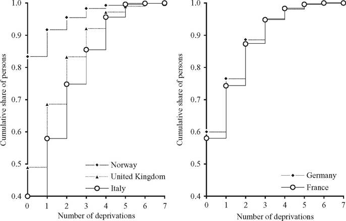
Figure 3.1 Cumulative distributions of material deprivation scores in selected European countries in 2012. Source: authors' elaboration on data from Eurostat (2014).

Table 3.2 Distribution of material deprivations in selected European countries in 2012 (percentage of total population)

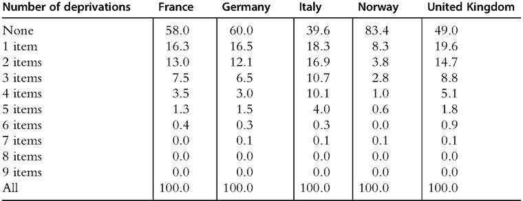
Source: Eurostat (2014).

deprivation in, at most, the number of dimensions indicated on the horizontal axis. (Figure 3.1 considers a maximum of seven deprivation items because nobody suffers from more than seven in the countries considered.) The left panel shows that Norway first- degree dominates both the United Kingdom and Italy, whereas the last two countries cannot be ordered by the criterion of first-degree dominance because their distributions intersect. The United Kingdom clearly lies ahead of Italy for up to five items, but then it exhibits a share of people suffering from six or seven deprivations that is more than twice the Italian level (1% vs. 0.4%, see Table 3.2). The right panel of Figure 3.1 shows that the cumulative distributions of deprivation scores for France and Germany also intersect, though they are much closer. The share of nondeprived is higher in Germany than in France, and the same holds true when we sequentially add those with one, two, and three deprivations; however, when we add people suffering from four deprivations, the order reverses, and it no longer changes when we consider more severe situations.^[112]

This example shows that first-degree dominance might be too demanding in practice: where count distributions intersect, they can be ranked only by defining weaker dom­inance criteria. This implies that we have to impose stricter conditions on the preference ordering of the social evaluator, taking into account that, in the study of deprivation, we might be leaning toward either the intersection or the union criteria. In the former case, we would start aggregating “from above,” looking first at the proportion of those who are deprived in r dimensions, then adding the proportion of those failing in r — 1 dimensions, and so forth; in the latter case, we would start “from below.” This distinction naturally leads to the definition of two second-degree dominance criteria, as suggested by Aaberge and Peluso (2011):

Definition 3.2A

A deprivation count distribution F₁ is said to second-degree downward dominate a deprivation count 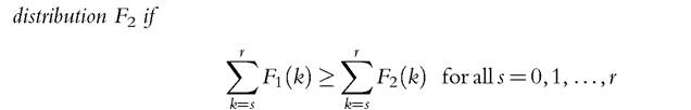and the inequality holds strictly for some s.

Definition 3.2B

A deprivation count distribution F₁ is said to second-degree upward dominate a deprivation count distribution

and the inequality holds strictly for some s.

If F₁ second-degree dominates F₂, then F₁ exhibits less deprivation than F₂, as before, but this result is now obtained at the cost of imposing the stricter conditions on the pref­erence ordering that will be shown below by Theorems 3.1A and 3.1B. Moreover, we have to make a choice between being more concerned with the extent to which depri­vation is diffused across the population (union criterion) or the occurrence of multiple dep­rivations (intersection criterion). In the first case, we would adopt second-degree upward dominance. Intuitively, we can see this in Definition 3.2B from the fact that we are making comparisons on (doubly) cumulated population proportions that start by considering the share of people who do not suffer from any deprivation, F(0), and we sequentially add the shares of those who suffer from one deprivation, then those who suffer from two depri­vations, and so forth. In calculating the cumulative function we “go up.” The opposite happens in the second case, for which we aggregate “going down,” thus placing more weight on the most deprived. Formally, second-degree upward dominance parallels the dominance criterion used by Atkinson (1970) for ranking income distributions. Second-degree downward dominance has no correspondent in the income inequality lit­erature, because it would be inconsistent with the Pigou-Dalton principle of transfers. It is, however, analogous to the criterion introduced for Lorenz curves by Aaberge (2009).

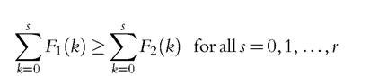
Is agreeing on whether to go up (union criterion) or to go down (intersection criterion) when we aggregate deprivation scores sufficient in empirical applications? Not always. This can be seen by reconsidering the previous comparisons of Italy and the United King­dom, and of France and Germany, with neither country in each comparison found to first- degree dominate the other. In Figure 3.2, we plot the difference between the integrated cumulative distributions considered by Definitions 3.2A and 3.2B for each pair of coun­tries. Ifwe integrate going up as in Definition 3.2B, the United Kingdom and Germany second-degree (upward) dominate Italy and France, respectively: the lower proportions of people who do not suffer from any deprivation give the first two countries an advantage that is not offset by their worst results for the incidence of people deprived in many dimen­sions. On the other hand, if we integrate going down as in Definition 3.2A, the difference between the integrated cumulative distributions changes from positive to negative, and no country second-degree (downward) dominates the other in either comparison. The dis­tribution of deprivation scores enables social evaluators favoring the union perspective to rank the United Kingdom and Germany ahead of Italy and France, but it does not allow social evaluators supporting the intersection perspective to draw unambiguous conclu­sions. In such a case, higher-degree criteria are needed, although they could still provide a partial ordering. The exploration of higher-order dominance criteria is a topic for further research. We turn instead to methods that can lead to a complete ordering.

3.3.2.2 Complete Orderings: The Independence Axioms

A complete ordering can be achieved by imposing an independence axiom for preference ordering. This allows us to weight differently certain parts of the distributions and even­tually to define a summary measure of deprivation. Formally, let social preferences be

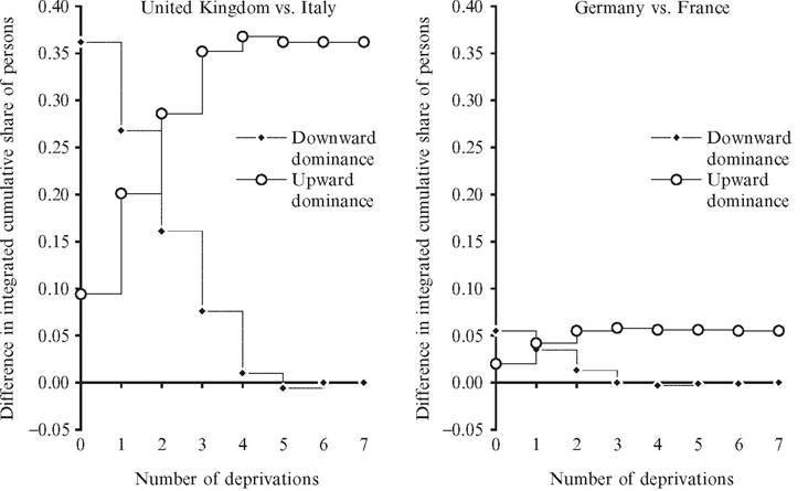
Figure 3.2 Second-degree dominance for material deprivation scores in selected European countries in 2012. Source: authors' elaboration on data from Eurostat (2014).

represented by the ordering^-defined on the family of deprivation count distributions F. This preference ordering is assumed to be continuous, transitive, and complete and to satisfy the condition of first-degree count distribution dominance. As proved by Debreu (1964), a preference ordering that is continuous, transitive, and complete can be represented by a continuous and increasing preference functional. We need further conditions to give social preferences an explicit empirical content, however. We there­fore introduce two alternative independence conditions, which require that the prefer­ence ordering is invariant with respect to certain changes in the count distributions being compared:

This axiom focuses on the proportions of people suffering from given numbers of deprivations (the F). We could instead focus on the number of deprivations that is asso­ciated with a given proportion of people, that is, more technically, the rank in the count distribution (the F^r1). This corresponds to an alternative version of the independence axiom, as in the literatures on uncertainty and inequality:

If F₁ is weakly preferred to F₂, then the independence axiom (similar to the expected utility theory) states that any mixture on F₁ is weakly preferred to the corresponding mix­ture on F₂: identical mixing interventions on the count distributions do not affect their ranking, which depends solely on how the differences between the mixed count distri­butions are judged. Thus, if the overall count deprivation is lower in country 1 than in country 2, so that F₁ F₂, the ranking would not change by adding to the population of either country the same group of migrants, whose deprivation distribution is F₃. The ordering relation is therefore invariant with respect to the aggregation of subpopula­tions across deprivations.

The dual independence axiom shifts toward aggregating subsets of deprivation dimen­sions across proportions of people. Assume that there are only two deprivation indicators, income and health, and that two alternative tax and benefit regimes produce the two count deprivation distributions F₁ and F₂ for income. Next, match F₁ with the count deprivation distribution F₃ for health in such a way that the most deprived person in income is also the most deprived person in health, the second most deprived person in income is the second most deprived person in health, and so on. Match F₂ and F₃ in the same way. If the count deprivation distribution F₁ is preferred to F₂ for income, then the share of income- deprived people under regime 1 is lower than the corresponding share under regime 2. Dual independence means that, given any distribution F₃ of health deprivation counts, F₁ will continue to be preferred to F₂ after matching both F₁ and F₂ with F₃. The dual independence axiom imposes this invariance property regardless of the shape of the count deprivation distribution for health (F₃) and of the weights used for such a matching (α).

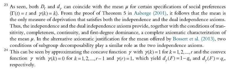
The essential difference between the two axioms is that the independence axiom deals with the relationship between a given number of deprivations and weighted averages of the corresponding population proportions, but the dual independence axiom deals with the relationship between given population proportions and weighted averages of the cor­responding numbers of deprivations. No one has so far provided a convincing justifica­tion for preferring one axiom to the other, but the choice of the axiom yields summary measures of deprivation with different decomposition properties. For instance, indices consistent with the independence axiom can be expressed as weighted averages of the corresponding indices computed for mutually exclusive population subgroups, whereas the indices satisfying the dual independence axiom cannot. By contrast, the dual measures offer a convenient decomposition by sources of deprivation, whereas the measures asso­ciated with the independence axiom cannot. Moreover, as measures of income

²¹ This argument parallels the rationale offered by Weymark (1981, p. 418) for his “Weak Independence of Income Source” axiom: “if in two income distributions the incomes from all but one type of income are the same in both distributions, then the overall judgement that one distribution is more unequal than a second is completely determined by a comparison of the distributions of income from the variable source.” Gajdos and Weymark (2005) call the corresponding multidimensional condition “Weak Como­notonic Additivity.” inequality, they have the convenient property of being expressed as linear functionals of the Lorenz curve, whereas the primal measures cannot.

The “primal approach,” based on the independence axiom, is analogous to the inequality framework developed by Atkinson (1970), and it parallels the discussion of the headcount curves by Aaberge and Atkinson (2013). The “dual approach,” based on the dual independence axiom, is analogous to the rank-dependent measurement of inequality introduced by Weymark (1981) and Yaari (1988) and to the way to summa­rization of the informational content of Lorenz curves by Aaberge (2001). In what fol­lows, we draw on Aaberge and Peluso (2011) for the dual approach and Aaberge and Brandolini (2014) for the primal approach.

3.3.2.3 Complete Orderings: The Dual Approach

The dual independence axiom can be used to justify the following family of deprivation

measures

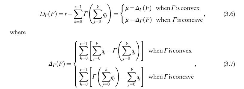
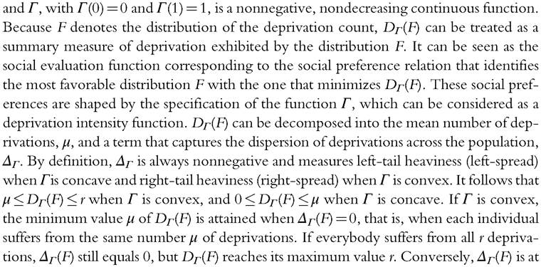
a maximum when half of the population does not suffer from any deprivation and the remaining half suffer from all, so that D_r(F) = r[1 — Γ(0.5)]. The comparison between the last two cases illustrates how the index works: a situation in which everybody suffers from r deprivations is definitely worse than one where only half of the population suffers from r deprivations. But the extent to which the two situations are valued differently depends on the convexity of Γ: the more convex it is, the more weight we give to mul­tiple deprivations, and the closer D_r(F) is to r. A similar reasoning applies, mutatis mutan­dis, for concave Ã.

Expression (3.6) shows that an exclusive concern for the mean number of deprivations implies linear (both convex and concave) social preferences: Γ(t) = t. There is indifference between a situation in which s people have one deprivation and a situation in which only one person is deprived but in s dimensions. It is the same result that we would obtain by applying the composite index approach discussed in Section 3.3.1, and it is another way to appreciate the restrictions imposed on social preferences in that approach. When there is a concern for the distribution of deprivations across the population, the critical judgement is whether this concern should prioritize the intensity or the diffusion of deprivations. In the former case, social preferences pay more attention to one person with s deprivations than to s people with one deprivation each, and the measure D_r should embody a convex Γ. In the latter case, social preferences take the opposite stance, and the measure D_r should embody a concave Γ. With Γ concave, for a given μ, D_r decreases as Δ_r increases because the distribution of deprivations across the population shifts towards people with none or fewer deprivations or, in other words, to the left tail of the distribution.

Thus, there is a correspondence between convexity and the intersection criterion on one side and between concavity and the union criterion on the other. This can be seen by taking particular specifications of the function r. With the union criterion, the focus is on the proportion of people who suffer from deprivation in at least one dimension (1 — q0). By specifying r as

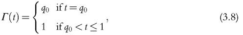
we get D_r(F) = 1 — q₀, which means that the union measure can be considered as a lim­iting case of the D_r-family of deprivation measures in the concave case. With the inter­section criterion, the focus is on the proportion of people deprived in all dimensions (q_r). The following alternative specification for r,

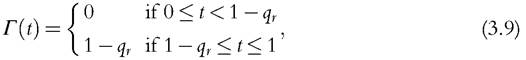
yields D_r(F) = r — 1 + q_r, which means that the intersection measure also represents a lim­iting case of the D_r-family of deprivation measures in the convex case. Although the union and intersection measures do not belong to the D_r-family, which is generated

3.3.2.4 Complete Orderings: The Primal Approach

The independence axiom provides a justification for the following alternative family of deprivation measures,

and γ(k), with γ(0) = 0, is a nonnegative, non-decreasing continuous function of the number of deprivations k. As with Γ in the dual case, γ can be considered as a deprivation intensity function with a curvature that determines how much we dislike increasingly severe deprivations in the convex case or growingly diffuse deprivations in the concave case. This family of deprivation measures is analogous to the family of inequality measures introduced by Kolm (1969) and Atkinson (1970). Chakravarty and D’Ambrosio (2006) provide an alternative axiomatic justification of (3.10) with a convex γ for measuring social exclusion.²²

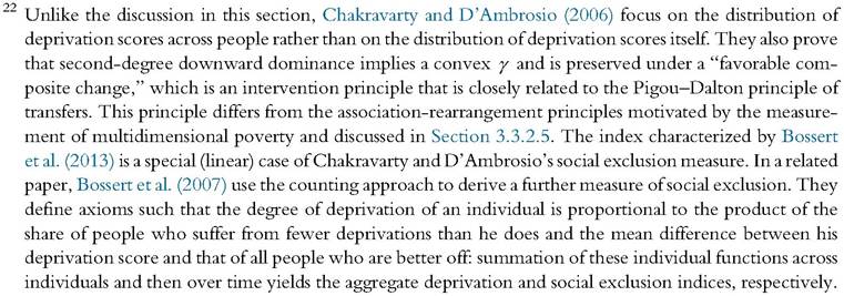
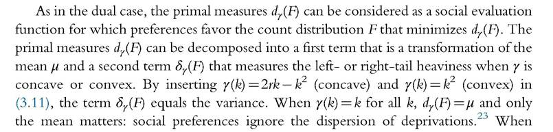
the dispersion matters, as in the dual case, the judgement depends on whether social pref­erences give more weight to s people with one deprivation each or to one person with s deprivations, which means choosing a concave function γ in the first case and a convex function in the second. Indeed, the union criterion is a limiting case of the d_γ -family of deprivation measures for concave γ, and the intersection criterion is a limiting case for

Unlike the dual measures, the primal measures are exactly decomposable by popula­tion subgroups, in the sense that the index computed for the overall population equals the weighted average of the measures calculated for each subgroup, with weights equal to the respective population shares of the subgroups. Note, that the dual measures may admit a different decomposition into within-group and between-group components, however, along the lines suggested by Ebert (2010).

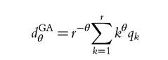
The measure d_γ generalizes the counting measure proposed by Atkinson (2003, p. 62) for a bivariate distribution (r=2). Atkinson’s measure A_θ can be written as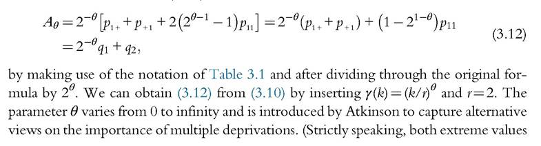

are inconsistent with the assumed continuity of the function γ, and they should be seen as limiting cases.) When θ→ 0, the index counts all people with at least one deprivation, regardless of their number for each individual:When

θ = 1, people with two deprivations are counted twice and A₁ gives the simple mean of the headcount rates in the two dimensions, providing the same result as would be gen­erated with a composite index. As θ goes to infinity, the index tends to coincide with the proportion of people deprived on both dimensions:. As the original Atkinson’s

counting deprivation index, its generalization to more than two dimensions obtained by insertingin (3.10) embodies, as limiting cases, both the union criterion (Ao)

and the intersection criterion (A₁). This index characterizes a family of deprivation mea­sures that may be seen as the analog of the poverty measures proposed by Foster et al. (1984), referred to as the FGT measures.

The decomposition of the primal and dual measures of deprivation in terms of mean (or transformation of the mean) and dispersion of the deprivation count distributions par­allels the mean-inequality decomposition of the social welfare functions derived from the expected and rank-dependent utility-like theories (see Atkinson, 1970; Yaari, 1988). Unlike the income inequality analysis, the structure of the decomposition of the depri­vation measures depends on whether social preferences are associated with the union or the intersection criterion, however. In the former case, the deprivation measures fall and social welfare rises when the dispersion of deprivation across the population goes up, meaning that more people are affected by few or no deprivations. Even though they allow for the decomposition in terms of mean dispersion of deprivation, the primal and dual summary measures are silent about the role played by each dimension. Thus, the information provided by these summary measures should be complemented with estimates of the proportions of people who suffer from deprivation in each of the dimen­sions. This information reveals whether deprivation is concentrated on few or many dimensions.

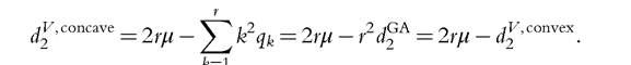
Table 3.3 shows the estimates for some deprivation indices for the five European countries considered earlier. (Some indices are discussed in the next sections.) As regards dual measures, we consider the class of indices associated with the Lorenz family of inequality measures,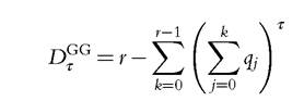

for various values of the parameters τ. For τ = 2, the previous expression gives the convex version of the Gini-type measure of deprivation, and the concave version is given by: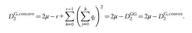

Table 3.3 Indices of material deprivations in selected European countries in 2012

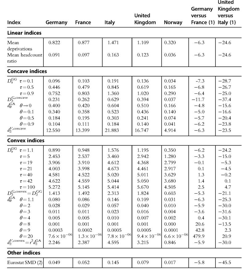
Note: (1) Percentage relative deviation of the figure for the first country from the figure for the second country.

(2) Figures are computed from Table 3.2 and may differ from published statistics because of rounding.

Source: authors' elaboration on data from Eurostat (2014).

In regard to primal measures, we consider the generalized Atkinson-type class of indices

for various values of the parameters θ. For θ = 1, the previous expression gives the mean headcount ratio, which equals the ratio μ7r. For θ = 2, it coincides with the convex ver­sion of the variance-type measure of deprivation d^v,convex multiplied by r ², and the con­cave version

Norway shows the lowest mean number of deprivations followed by Germany and France, which are rather close each other, the United Kingdom, and finally Italy. The mean headcount ratio ranges from 3.6% in Norway to 16.3% in Italy. With a con­cave index, we always find that deprivation is lower in Germany than in France and lower in the United Kingdom than in Italy, which is not surprising in light of the results on second-degree upward dominance reported in Section 3.3.2.1. On the other hand, the lack of second-degree downward dominance in these same comparisons is notice­able in the fact that the rankings reverse as the functions become more convex. For instance, the generalized Atkinson-type deprivation index turns out to be lower in France than in Germany for values of θ higher than 4. The French overall deprivation is below the German level whenever we favor the intersection criterion and weight somebody suffering from 2h deprivations at least 16 (=2⁴) times somebody suffering from h deprivations (as the indexassigns each person with h deprivations a weight equal to h⁴). Because the United Kingdom fares much better than Italy, except in the occurrence of very severe deprivation (6 or more items), the ranking between the two countries only changes for high values of θ or τ, which correspond to an extreme aver­sion to the worst conditions of deprivation. Finally, note that the generalized Atkinson- type deprivation index approaches the proportion of people experiencing at least one deprivation (union criterion) as θ tends to 0, and the proportion of people suffering from the maximum number of deprivations (intersection criterion) as θ goes to infinity; as nobody lacks all nine items, in the latter case, the index converges to zero in all countries.

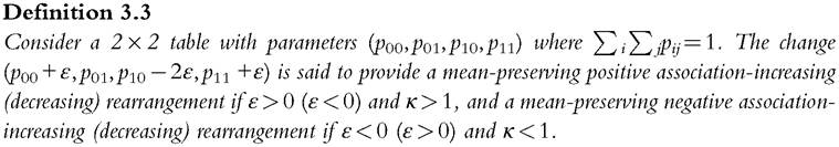
3.3.2.5 Association Rearrangements

In many respects, the discussion so far has proceeded as in the case of a single variable, whereas the key feature of the multivariate case is the pattern of association across dimensions. It is then natural to ask how social welfare responds to a change in the

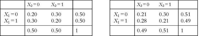
Table 3.4 Illustration of a marginal-free positive association-increasing rearrangement

Source: authors' elaboration.

Table 3.5 Illustration of a marginal-free negative association-increasing rearrangement

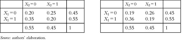
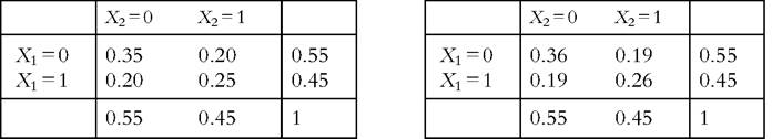
distribution of deprivations across the population, although the total number of depri­vations remains the same. The standard approach is to consider how social welfare varies after a “marginal-free change” in the association between two variables, which is a change that does not affect the marginal distributions. As in the statistical literature on the measurement of association in multidimensional contingency tables (formed by two or several binary variables), we distinguish association rearrangements for dis­tributions characterized by either positive or negative associations. Illustrations of marginal-free association rearrangements are provided by Tables 3.4 and 3.5. Each panel of Table 3.4 is obtained from the opposite panel by a marginal-free positive association-increasing (decreasing) rearrangement, whereas each panel of Table 3.5 can be obtained from the opposite panel by a negative association-increasing (decreas­ing) rearrangement.

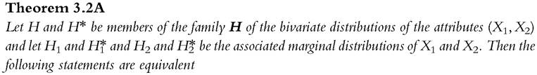
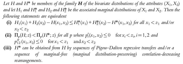
Marginal-free rearrangements have been widely used as a basis for evaluating multi­dimensional measures of poverty and inequality.^[113] Bourguignon and Chakravarty (1999, 2003, 2009) and Atkinson (2003) use the principle of marginal-free correlation­increasing shifts as a basis for making a normative judgement of poverty measures derived from continuous variables (attributes) rather than from deprivation scores. They distin­guish whether the poverty measure increases or decreases because of a correlation­increasing shift, and they consider the associated attributes to be substitutes (one attribute can compensate for the lack of the other) in the former case and to be complements in the latter.

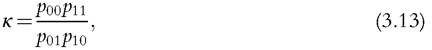
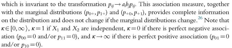
Considering marginal-free changes is a neat way to highlight the fact that the multi­dimensional analysis of poverty and inequality implies making assumptions regarding the degree to which the different attributes can be substituted one for the other. In the real world, the condition of marginal-free changes may be too restrictive because policies may reduce deprivation in one dimension at the cost of increasing deprivation in another. We hence adopt a more general approach, and we require that only the mean number of deprivations but not the marginal distributions be kept fixed. (The latter implies the for­mer, but not vice versa.) It follows that we need a measure of association that is invariant with regard to changes in the marginal distributions, unlike the correlation coefficient. This is the case of the cross-product κ introduced by Yule (1900). In the 2 ? 2 distribution of Table 3.1, Yule’s measure is defined by

Following Aaberge and Peluso (2011) and Aaberge and Brandolini (2014), we relax the marginal-free condition by introducing an association-increasing/decreasing rearran­gement principle that relies on the condition of a fixed overall mean number of depri­vations rather than on the condition of fixed proportions of people suffering from each deprivation. As illustrated by Tables 3.4 and 3.5, marginal-free arrangements are special cases of this alternative rearrangement principle.²⁷

It follows from Definition 3.3 that a (mean-preserving rearrangement reduces the number of people deprived according to indicator X₁ at the cost of increasing the number of people deprived according to indicator X₂ when ε > 0 and vice versa when ε < 0. This is illustrated in Table 3.6, which shows two distributions where the association is negative (κ < 1) and the mean is equal to 1. Each panel can be obtained from the opposite panel by a mean-preserving negative association-decreasing (increasing) rearrangement where ε = 0.01.

Aaberge and Peluso (2011) show how to extend Definition 3.3 to r dimensions. As is the standard, subscript notation becomes cumbersome for more than two dimensions, so they simplify the notation to p_ij_m, where i and j represent two arbitrary chosen deprivation dimensions and m represents the remaining r — 2 dimensions. The Yule’s measure κ_ij_m is defined by

where m is an (r — 2)-dimensional vector of any combination of zeroes and ones. In this case, the association is defined by r(r —1)/2 cross-products. Aaberge and Peluso (2011) introduce the following generalization of Definition 3.3:

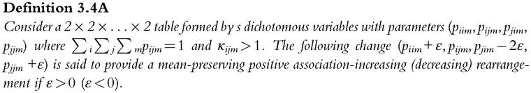
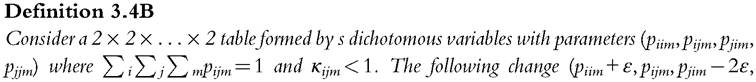
Table 3.6 Illustration of a mean-preserving negative association-decreasing rearrangement

Source: authors’ elaboration.

Theorem 3.1A demonstrates that social preferences favoring second-degree down­ward dominance imply that overall deprivation rises after a mean-preserving positive association-increasing rearrangement, as well as a mean-preserving negative association-decreasing rearrangement, irrespective of whether preferences are consistent with the primal or the dual approach. By contrast, Theorem 3.1B proves that prefer­ences favoring upward second-degree dominance consider such rearrangement as a reduction in the overall deprivation. Moreover, it follows directly from the decompo­sitions (3.6) and (3.10) that the principles of mean-preserving association-increasing/ decreasing rearrangement are equivalent to the mean-preserving spread/contraction defined by:

Definition 3.5

me on- F1)

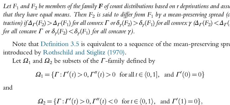
ad

and let ω₁ and ω₂ be subsets of the /-family defined by

and

All members of the sets Ω₁ and ω₁ are increasing convex functions, and all members of Ω2 and ω₂ are increasing concave functions.

Theorem 3.1A

Let F₁ and F₂ be members of the family F of count distributions based on r deprivations and assume that they have equal means. Then the following statements are equivalent:

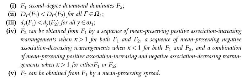
Theorem 3.1B

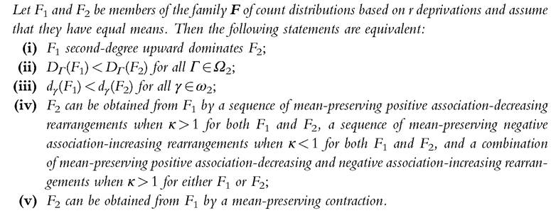
See Aaberge andPeluso (2011) Ioraproofofthe equivalence between (i), (ii), and (iv) of Theorems 3.1A and 3.1B, and Aaberge and Brandolini (2014) for a proof of the equiv­alence between (i) and (iii). The equivalence between (v) and (ii) and (iii) follows directly from the second terms of Equations (3.6) and (3.10).

Following the distinction made by Bourguignon and Chakravarty (2003, 2009) and Atkinson (2003), the results of Theorem 3.1A (3.1B) justify the use of D_γ and d_γ for con­vex Γ and convex γ (concave Γ and concave γ) when the attributes associated with the deprivation indicators can be considered as substitutes (complements). Theorems 3.1A and 3.1B show that D_γ and d_γ satisfy the mean-preserving association-rearrangement principles, when a distinction has been made between whether an association rearrange­ment comes from a distribution characterized by a positive or negative association. Con­sider the specific subfamily of two-dimensional deprivation measures discussed by Atkinson (2003) and defined by (3.12), and assume that there is positive association between the two deprivations (κ > 1). The d_γ-function associated with the family A_θ is concave for θ < 1 and convex for θ > 1, and it approaches the union condition when θ→ 0 and the intersection condition when θ→∞. Theorem 3.1B states that a sequence of mean-preserving positive association-decreasing rearrangements raises the overall

observe a reduction in the positive association between deprivations in the two attributes? After all, the share of people suffering from deprivation for both attributes falls, while the total number of deprivations does not vary. The answer is positive if we regard the two attributes as complements, which means that we rule out any trade-off between them, and we dislike the fact that more people are deprived more than the fact that fewer people are hit more.

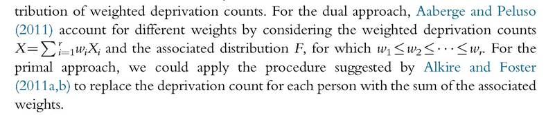
Until now, we have not considered the cases of unequal weighting of the dimensions. However, all results summarized by Theorems 3.1A and 3.1B remain valid for the dis-

3.3.2.6 Counting Deprivations versus Measuring Poverty

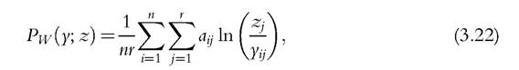
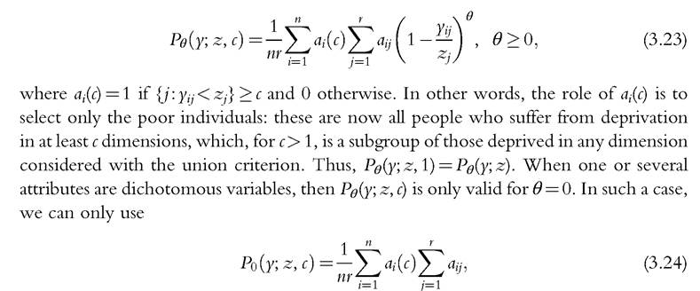
So far, we have been concerned with the distribution of deprivation counts, irrespective of how many people are regarded as poor when deprivation and poverty are considered as distinct concepts. In terms of the classical distinction made by Sen (1976), we have focused only on the aggregation of the characteristics of deprivation into an overall mea­sure of deprivation, ignoring the first step concerning the identification of the poor. The contrast between the union and the intersection criteria emphasized in the previous sec­tions suggests, however, that there is some leeway in defining who is poor. For instance, Brandolini and D’Alessio (1998), Bourguignon and Chakravarty (1999, 2003), Tsui (2002), and Bossert et al. (2013) adopt the more extensive union criterion and define people as (multidimensional) poor if they suffer from at least one deprivation. In this case, deprivation and poverty come to coincide. On the other hand, (the European Union regards as multiply materially deprived all persons who cannot afford at least four out of nine amenities, moving midway between the union and the (strict) intersection views. Alkire and Foster (2011a,b) formalize what they label the “dual cut-off’ identification system, in which the dimension-specific thresholds are integrated with a further threshold that identifies the minimum number of deprivations required for an individual to be clas­sified as poor. If a person is poor when he or she is deprived in at least c, 1 ≤ c ≤ r, dimen­sions, the headcount ratio is uniquely determined by the count distribution F and is defined by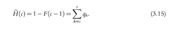

In the case of the European indicator of severe material deprivation, c equals 4. As the choice of a specific cut-off c is arbitrary, it is useful to check the sensitivity of the ranking of distributions to c by treating H(c) as a function of c, henceforth labeled the headcount curve. As is evident from (3.15), the condition of first-degree dominance of headcount curves is equivalent to first-degree dominance of the associated count distributions. If c > 1, first-degree dominance for headcount curves is a less demanding condition than that for the overall count distribution, because it ignores what happens to those who suf­fer from deprivation in fewer than c dimensions. Moreover, the second-degree domi­nance results of Theorems 3.1A and 3.1B are also valid for the headcount curve, which means that H(c) satisfies the principle of association-increasing/decreasing rear­rangements when this principle is restricted to be applied among the poor.

To complement the information provided by the headcount ratio when only ordinal data are available, we may employ the measures defined by (3.6) and (3.10) as overall measures of poverty for the conditional count distribution F defined by

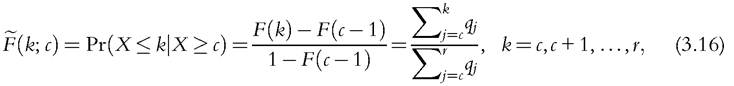
with mean given by

Expressions (3.6) and (3.10) show that the overall measures of poverty foradmit a decomposition into the mean (or a function of the mean) and a measure of dispersion. An analog to the FGT family of poverty measures is obtained by insertingin

expression (3.10).

As an alternative, Alkire and Foster (2011a) propose combining the headcount ratio and the conditional meanand they introduce the adjusted headcount ratio defined by

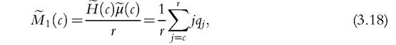
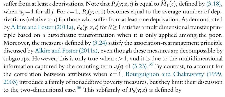
weights. Alkire and Foster (2011a, p. 482) underline that both the identification of the poor and the adjusted headcount ratio are invariant to monotonic transformations applied to the deprivation variables and the respective thresholds. Moreover, the index M ₁(c) increases if a poor person becomes deprived in an additional dimension (dimensional monotonicity), and it is decomposable by population subgroups. Therefore, the index can be broken down by indicator because it is the (weighted) average of the deprivations headcount ratios for each dimension computed considering only the poor at the numer­ator (so-called “censored headcount ratios”). On the other hand, this index is indifferent to changes in the way deprivations are distributed across the poor.²

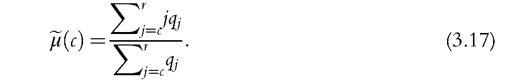
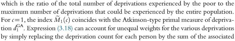
A general family of adjusted poverty measures that take into account not only the average deprivation experienced by the poor, μ(c), but also the distribution of depriva­tions across the poor can be derived from the d-measure defined by (3.10)

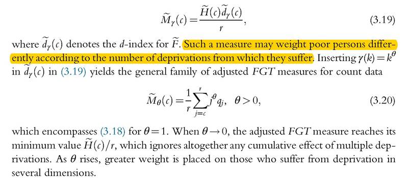
Figure 3.3 compares how poverty headcount ratios change as we vary the poverty cut-off using the deprivation indicators in the five European countries considered earlier. The proportion of poor people, shown in the top-left panel, falls by three-fourths in Italy and around nine-tenths in the other countries as the poverty cut-off is raised from one deprivation (union criterion) to four deprivations (the European criterion). Censoring at four deprivations implies excluding from measured poverty a substantial fraction of the population suffering from one, two, or three deprivations: 15% in Norway and 46% in Italy, accounting for 76% and 57% of all deprivations, respectively. However, the ranking ^[114]

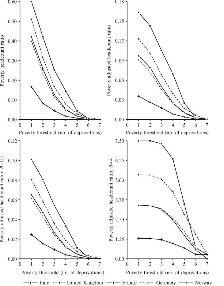
Figure 3.3 Poverty headcount and adjusted headcount ratios fordιfferent poverty cut-offs in selected European countries in 2012. Source: authors' elaboration on data from Eurostat (2014).

of countries does not change. It changes when the cut-off is set at five deprivations, how­ever, when Germany and France reverse their order, and again at six deprivations, when the United Kingdom becomes the country with the highest share of poor people. In the top-right panel, the ranking is the same for the adjusted headcount ratio M 1 (c), except for a better position granted to France by its lower average intensity of deprivation (μ(c)/r) when the cut-off is set at six deprivations. The bottom panels show results for the adjusted FGT measure M θ (c): lowering the weights of multiple deprivations (θ = 0.5; left panel) does not modify the sorting produced by the adjusted headcount ratio, whereas signif­icantly raising them (θ = 4; right panel) steadily switches the positions of Germany and France, as seen in Section 3.3.2.4. This comparison reveals that varying the poverty cut­off has a considerable impact on measured poverty, whereas adjusting the headcount ratio for the deprivations experienced by the poor seems to have minor effects, unless their distribution is taken into account.

The adjusted headcount ratioproposed by Alkire and Foster (2011a,b) pro­vides the theoretical basis for the Multidimensional Poverty Index (MPI) developed by Alkire and Santos (2010, 2013, 2014).²⁹ The MPIhas replaced the HPIin the reports of the United Nations Development Program since 2010 in order to capture “how many people experience overlapping deprivations and how many deprivations they face on average” (UNDP, 2010, p. 95). The MPIconsiders 10 dichotomous indicators for three dimensions: health, education, and living standards. Dimensions and indicators within each dimension are equally weighted, and the cut-off c for the number of (weighted) dep­rivations is set at three out of a maximum of ten. Applied research estimating Alkire and Foster’s class of indices and the MPI is rapidly growing.³⁰

3.3.3 Poverty Measurement Based on Continuous Variables

The counting approach focuses on the distribution of deprivation scores that summarize binary variables, defined as having or not having goods or performing or not performing activities that are seen as social necessities. When we have cardinal (continuous or cat­egorical) variables, we can use measures of multidimensional poverty that fully exploit

²⁹ Alkire and Foster’s method is utilizedby Peichl and Pestel (2013a,b) to derive an adjusted headcount ratio for multidimensional richness. This index accounts for the number of individuals who are affluent in a minimum number of dimensions, as well as for their average achievements in these dimensions.

³⁰ See for instance, Roelen et al. (2010) for Vietnam, Khan et al. (2011) for Pakistan, Batana (2013) for Sub-Saharan African countries, Battiston et al. (2013) for Latin American countries, Roche (2013) for Bangladesh, Santos (2013) or Buthan, Trani, and Cannings (2013) for Western Darfur, Trani et al. (2013) for Afghanistan, Yu (2013) for China, and Cavapozzi et al. (2013) and Whelan et al. (2014) for European countries. See also Mohanty (2011) for a related study on deprivation scores in India. Bennett and Mitra (2013) develop multiple statistical tests for Alkire and Foster’s family of poverty measures. the informational richness of the available data.^{[115] [116]} As in the counting approach, we may aggregate attributes first across dimensions and then across individuals. This procedure corresponds to representing each individual’s vector of attributes with an interpersonally comparable utility-like function and then evaluating the distribution of individual well­being using the same tools as in a univariate space. Consumer theory (Slesnick, 1993) or information theory (Maasoumi and Lugo, 2008) can provide the analytical framework to derive the utility-like function. This function is then used to aggregate the attribute­specific cut-offs to define an aggregate poverty threshold.^[117]

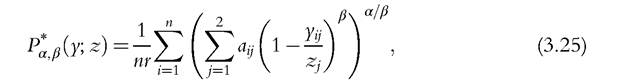
Alternatively, we may employ an axiomatic simultaneous aggregation approach for measuring multidimensional poverty. Chakravarty et al. (1998), Bourguignon and Chakravarty (1999,2003), and Tsui (2002) consider persons to be poor ifthey suffer from at least one deprivation (the union approach), whereas Alkire and Foster (2011a) take all those who are deprived in at least c dimensions, with c between 1 and r. All these papers then aggregate the individual shortfalls relative to dimension-specific cut-offs into a mul­tidimensional poverty measure. The actual functional forms of the poverty indices are determined by the combination of chosen axioms, many of which parallel those consid­ered in the univariate analysis (e.g., Zheng, 1997). In the next section, we selectively review these indices and illustrate some of their properties. We refer to Chakravarty et al. (1998), Bourguignon and Chakravarty (1999, 2003), Tsui (2002), and Chakravarty and Silber (2008) for proofs and further discussion of the axioms.

where a_ij is equal to the weight Wj assigned to attribute j if y_ij < Zj and to 0 otherwise; both a_ij and θj determine the weight assigned to attribute j in the poverty index.^{[118] [119]}

In addition to displaying monotonicity, continuity, and scale invariance, the members of the family P_θ(y; z) satisfy three axioms worthy of some comments. Subgroup decomposabil­ity requires that overall poverty can be expressed as a weighted sum of the poverty ratios of the subgroups and implies that the poverty index is separable across individuals. Thanks to this property, the poverty index identifies an individual poverty function. The one­dimensional Pigou-Dalton transfer principle demands that poverty does not increase in the case of a progressive transfer of one unit of attribute j from one poor person to a poorer person. This axiom determines the additivity of (3.21) across attributes. This factor decom­posability may be a useful feature because it allows identifying the contribution of each attribute to the overall poverty level.

The focus axiom highlights the greater complexity of multidimensional analysis. In the univariate income case, it simply entails that the poverty index is independent of the dis­tribution of income among the nonpoor. In the multivariate case, it may require the pov­erty measure to be invariant with respect to increases in y_ij if y_ij > Zj for all i, poor and nonpoor alike (strongfocus), or only with respect to changes in the distribution of attributes among the nonpoor (weakfocus). The stronger version of the axiom implies that a better achievement in a dimension in which an individual is not deprived cannot compensate for a below-threshold achievement in another dimension. The possibility of trading off one attribute for the other is ruled out. This is the case of (3.21), as a_ij equals 0 if y_ij > z_j∙.³4

The family of poverty measures P_θ(y; z) is a particular specification of the more gen­eral class characterized by Chakravarty et al. (1998) and Bourguignon and Chakravarty (1999, 2003) in which the power function is replaced by a continuous nonincreasing convex function. Assuming that all attributes are positive and specifying such a function to be the negative of the logarithm, Chakravarty and Silber (2008) and Chakravarty et al. (2008) obtain the multidimensional version of the poverty index proposed by Watts (1968) and formalized by Zheng (1993):

As indicated by Bourguignon and Chakravarty (2003) and Pattanaik et al. (2011), the measures defined by (3.21) are not sensitive to association-rearrangement interventions.

This is due to the fact that P_θ(y; z) is uniquely determined by the marginal distributions of the r attributes and the associated attribute-specific poverty thresholds. By imposing an additional condition, called the poverty focus axiom, Alkire and Foster (2011a) provide a justification for the intermediate poverty measure analog to P_θ(y; z),

which is equal to the average number of deprivations (normalized by the maximum num­ber r) experienced by the poor, or the normalized average among those individuals who

³⁵ As before, the introduction of the threshold can be criticized because it implies ignoring the condition of those who suffer from deprivation in less than c dimensions as well as because of the arbitrariness of the choice of c.

³⁶ For alternative families of multidimensional poverty measures and their characterizations, we refer to Kolm (1977), Chakravarty et al. (1998), Tsui (2002), Deutsch and Silber (2005), Duclos et al. (2006a, 2007, 2008), Chakravarty and Silber (2008), and Lasso de la Vega and Urrutia (2011). Diez et al. (2008) and Chakravarty and D’Ambrosio (2013) derive subgroup-decomposable multidimensional pov­erty indices that are unit-consistent; that is, they provide poverty rankings that are unaffected by a change in the measurement units of dimensions.

where α and β are nonnegative parameters, and it is used by Bourguignon and Chakravarty (1999, 2003) and Atkinson (2003) as a basis for demonstrating that the effect of an increasing association (correlation) rearrangement depends on whether the attri­butes are substitutes or complements, and that this corresponds to choosing α > β or α < β. Moreover, Atkinson (2003) demonstrates that the family of counting measures A_θ defined by (3.12) can be seen as a limiting case of (3.25) when α and β tend to zero with θ = à/â and w₁ = w₂ = 1.

3.3.3.2 Partial Orderings

Most empirical studies consider few measures of poverty when ranking multidimensional distribution functions. A natural concern is that the conclusions reached in these studies are sensitive to the choice of the specific measures.^{37 [120] [121] 39} By drawing on Atkinson and Bourguignon (1982), Bourguignon and Chakravarty (2009) investigate what restrictions two alternative stochastic dominance conditions of the first-degree impose on the general family of two-dimensional poverty measures defined by

where H is the bivariate distribution of the two attributes in question and p(x₁, x₂; z₁, z₂) is the level of poverty associated with attribute levels (x₁, x₂) and poverty thresholds (z₁, z₂). ⁹ Let p_i denote the derivative ofp with respect to x_i and let p"₂ denote the second derivative ofp with respect to x₁ and x₂.The following alternative presentation of a result from Bourguignon and Chakravarty (2009) provides three equivalent statements:

^[1] Brandolini (2009) and Madden (2011) use this index to study income and health poverty in selected European countries, and they analyze the sensitivity of results to different values of the parameters α and β. See also Bibi and El Lahga (2008).

The equivalence between (i) and (ii) is proved by Bourguignon and Chakravarty (2009), and the equivalence between (ii) and (iii) is proved by Atkinson and Bourguignon (1982).

Theorem 3.2A shows that poverty measures Π_p that satisfy condition (ii) rank bivar­iate distributions according to first-degree stochastic dominance for attribute values below the poverty threshold in each dimension and first-degree two-dimensional sto­chastic dominance below both poverty thresholds. As indicated by Bourguignon and Chakravarty (2003, 2009), and demonstrated by Theorem 3.2A, the principle of correlation-increasing rearrangement (conditional on fixed marginal distributions) is associated with the intersection H(x₁,x₂). Moreover, Theorem 3.2A shows that Π_p increases as a result of correlation-increasing rearrangement if the cross-derivative of p with respect to x₁ and x₂ is nonnegative. This is the reason why Bourguignon and Chakravarty, in this case, refer to the attributes as substitutes. The case in which the cross-derivative is negative corresponds to complements that are associated with nonincreas­ing poverty under a correlation-increasing rearrangement. An alternative presentation of this result is given by the following theorem:

Theorem 3.2B

For the proof of Theorem 3.2B, we refer to Atkinson and Bourguignon (1982) and Bourguignon and Chakravarty (2009). Note that Theorems 3.2A and 3.2B are, strictly speaking, only valid in cases for which the association (correlation) between X₁ and X₂ is positive. However, as demonstrated for the counting approach (see Theorems 3.1A and 3.1B), it is straightforward to extend Theorems 3.2A and 3.2B to cover the case in which the association (correlation) is negative.

In practice, multivariate distributions might often cross. This is shown, for instance, by Arndt et al. (2012) and Nanivazo (2014) in their multidimensional analyses of first order dominance for child poverty in Vietnam and Mozambique and in the Democratic Republic of Congo, respectively. Thus, it is helpful to introduce weaker criteria than first-degree dominance. Duclos et al. (2006a, 2007, 2008) consider second-degree and higher-degree dominance conditions when attributes are regarded as substitutes. A good example is when we consider poverty in relation to both income and wealth, which are perfect or very close substitutes. (Imperfect substitutability may derive from the lower degree of liquidity of an asset.) In these exercises, the asset poverty line is often defined with reference to the income poverty line, because it is taken to be the amount of wealth necessary to maintain the socially defined minimum standard for a certain period for someone who has no other economic sources (e.g., Brandolini et al., 2010; Haveman and Wolff, 2004). Bourguignon and Chakravarty (2009) remark that this approach gets close to the unidimensional approach because the poverty line of one attribute is assumed to be a function of the poverty line of the other attribute.

3.4.