Public expenditure
In this chapter we consider the growth of public expenditure and the difficulties surrounding its control. The next chapter will examine the burden of taxation. Given the key policy objectives in the UK of eliminating the budget deficit by 2014/15 and with 70% of the adjustment to take the form of public expenditure restrictions, this chapter and Chapter 19 on taxation assume even greater importance.
Here we look at public expenditure, its form, size and apparently inexorable growth. Problems of definition and calculation are considered, as resolving such ambiguity is extremely important since entire economic and political platforms rest upon the outcome. Attempts to control public expenditure are nothing new; they began early in the nineteenth century, long before Gladstone. Whatever the definition used, successive governments have had difficulty in controlling public expenditure, and the most widely used ratio of public expenditure (Total Managed Expenditure) to GDP has risen from 36.4% in 2000 to 47.2% in 2009/10. The major rise in this ratio has occurred in the period since 2007, with government interventions to offset global recession combining with already planned increases in public expenditure to raise this ratio from 41.1% in 2007/08 to 47.2% in 2009/10. The intention in the Comprehensive Spending Review of October 2010 is to bring this ratio down to 40% by 2015 and to reduce the current public sector net cash requirement (previously PSBR) from 11% to zero.
Trends in UK public spending
Figure 18.1 and Table 18.1 trace the relative importance of public expenditure in the UK economy between 1970 and 2010. Figure 18.1 shows Total Managed Expenditure (TME), previously called general government expenditure (GGE), as a percentage of GDP over an extended period of time in order to understand the changing role of the government in the economy.
This ratio rose sharply during the problem periods of the 1970s and 1980s when the UK economy suffered as a result of major oil shocks, but then the ratio fell during the growth years of the mid- to late 1980s and the period 1993-2007. Nor was it only growth in national income which contributed to the reduction in the ratio! The Conservative government was determined that public spending should take a declining share of GDP and announced severe cuts in public expenditure in November 1993, arguing that cuts in expenditure would lower government borrowing which, combined with lower taxation, would increase economic efficiency and improve the ‘supply side’ of the economy.When the Labour Party came to power in 1997, the ratio began to rise again for two main reasons: first, the Labour Party’s philosophical ideology as regards a more interventionist role for government in the economy; second, there was a backlog of projects which the new government believed needed attention. Whilst reluctant to change the previous Conservative government’s spending projections during its first five years in office (1997-2002), the Labour government undertook a major Comprehensive Spending Review in November 2002 which resulted in sharp increases in public spending over the period 2002/032005/06, with the average annual growth of spending over this period to be as follows: Transport (8.4%), Health (7.3%) Education (5.7%) and Housing (3.5%), all well above the projected 2% annual rate of inflation.
However, the ratio of public expenditure (TME) to GDP rose still more rapidly after 2007 as the effects of the credit crunch and the required government intervention to stabilize the economy coincided with additional expenditures planned in the last few years of that government. This rise has now been reversed with the Comprehensive Spending Review of the incoming Coalition government in 2010 projecting a significant reduction in the growth of public spending.
I Total Managed Expenditure (TME)
The Economic and Fiscal Strategy Report in June 1998 reformed the planning and control regime for public spending.
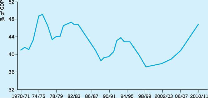
Fig.
18.1 Total Managed Expenditure (TME) as a percentage of GDP since 1970. Source: Adapted from HM Treasury (2010) Public Expenditure Statistical Analyses.Table 18.1 Historical series of government expenditure (% of GDP).
| Public sector current expenditure | Public sector net capital expenditure | General government expenditure (GGE) | Total Managed Expenditure (TME) | |
| 1970-71 | 32.7 | 6.2 | 41.0 | 42.7 |
| 1971-72 | 33.4 | 5.3 | 41.3 | 42.6 |
| 1972-73 | 33.2 | 4.9 | 40.8 | 41.9 |
| 1973-74 | 35.0 | 5.2 | 41.3 | 44.3 |
| 1974-75 | 38.7 | 5.6 | 47.6 | 48.6 |
| 1975-76 | 39.7 | 5.6 | 45.6 | 49.7 |
| 1976-77 | 39.7 | 4.4 | 45.6 | 48.5 |
| 1977-78 | 38.3 | 3.0 | 42.4 | 45.6 |
| 1978-79 | 38.2 | 2.5 | 43.0 | 45.1 |
| 1979-80 | 38.1 | 2.3 | 43.0 | 44.6 |
| 1980-81 | 40.6 | 1.9 | 46.0 | 47.0 |
| 1981-82 | 42.3 | 1.0 | 46.7 | 47.7 |
| 1982-83 | 42.3 | 1.6 | 46.6 | 48.1 |
| 1983-84 | 42.0 | 1.8 | 45.5 | 47.8 |
| 1984-85 | 42.2 | 1.6 | 45.5 | 47.5 |
| 1985-86 | 40.5 | 1.2 | 43.5 | 45.0 |
| 1986-87 | 39.7 | 0.7 | 41.6 | 43.6 |
| 1987-88 | 38.1 | 0.6 | 39.8 | 41.6 |
| 1988-89 | 35.8 | 0.3 | bgcolor=white>37.238.9 | |
| 1989-90 | 35.3 | 1.2 | 38.3 | 39.2 |
| 1990-91 | 35.6 | 1.3 | 38.5 | 39.4 |
| 1991-92 | 38.0 | 1.8 | 40.8 | 41.9 |
| 1992-93 | 39.8 | 1.8 | 42.8 | 43.7 |
| 1993-94 | 39.7 | 1.4 | 42.9 | 43.0 |
| 1994-95 | 39.3 | 1.4 | 42.2 | 42.5 |
| 1995-96 | 38.7 | 1.4 | 42.1 | 41.8 |
| 1996-97 | 37.6 | 0.7 | 40.3 | 39.9 |
| 1997-98 | 36.2 | 0.6 | 39.1 | 38.2 |
| 1998-99 | 35.2 | 0.7 | 38.3 | 37.3 |
| 1999-00 | 34.5 | 0.6 | 38.0 | 36.4 |
| 2000-01 | 35.0 | 0.5 | - | 36.8 |
| 2001-02 | 35.5 | 1.2 | - | 38.0 |
| 2002-03 | 36.1 | 1.3 | - | 38.7 |
| 2003-04 | 36.8 | 1.3 | - | 39.4 |
| 2004-05 | 37.6 | 1.7 | - | 40.6 |
| 2005-06 | 38.2 | 1.8 | - | 41.3 |
| 2006-07 | 37.7 | 1.9 | - | 40.9 |
| 2007-08 | 37.8 | 2.0 | - | 41.1 |
| 2008-09 | 39.4 | 3.2 | - | 43.9 |
| 2009-10 | 41.4 | 3.8 | — | 47.2 |
Source: Adapted from HM Treasury (2010) Public Expenditure Statistical Analyses, and previous issues.
■ Overall plans were to use a new distinction between current and capital spending.
■ Firm three-year plans (Departmental Expenditure Limits, DELs) were to provide certainty and flexibility for long-term planning and management.
■ Spending outside DELs, which could not reasonably be subjected to firm three-year spending commitments, was to be reviewed annually as part of the Budget process. This Annual Managed Expenditure (AME) is also subject to constraints.
■ Large public corporations, not dependent on government grants, were to be given more flexibility.
■ Total Managed Expenditure (TME) was defined as consisting of DEL plus AME and was to be widely used as the overall measure of government expenditure (replacing general government expenditure - GGE).
Making a clear distinction between public sector current expenditure and capital expenditure is a key element in the government’s ‘golden rule’ (see below). A historical series for these various definitions is shown in Table 18.1.
The debate on the role of public expenditure continues. Nevertheless, the previous Conservative and Labour governments both accepted that, as a cornerstone of the medium-term financial strategy, they should squeeze inflation progressively out of the economy, through a close control of the rate of growth of public expenditure. Continuing fiscal rectitude is seen as important for a government committed to the Maastricht criteria for fiscal convergence (see Chapter 27). These include a 3% target for the overall ratio of public sector borrowing requirement (PSBR) (now public sector net cash requirement) to GDP, and a 60% target for the ratio of public debt to GDP.
Figure 18.2 provides a useful overview of the intentions of the Comprehensive Spending Review of October 2010 in reducing future real levels (at constant 2010/11 prices) of Total Managed Expenditure further below already reduced totals planned by the previous Labour government in its March 2010 budget. The remaining difference between projected TME expenditure and tax revenues (see Chapter 19) will need to be financed by borrowing, but the intention is to all but close the gap between the expenditure and revenue lines by the end of the current Parliament in 2015.
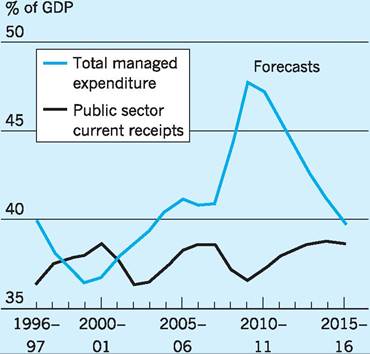
Fig. 18.2 Forecasts for spending and revenues. Source: Forecast for spending and revences % of GDP, Financial Times, 21/10/2010 (Wolf, M.).
Public spending and the National Debt
The National Debt has been reduced sharply by successive governments and at the start of the global recession of 2007/08 had fallen to around 50% of National Income. As can be seen from Fig. 18.3 this is well below the long-run average (1688-2010) of 112% of National Income.
However, the huge sums expended by the government since 2007 in order to rescue fundamentally insolvent financial institutions and purchase large
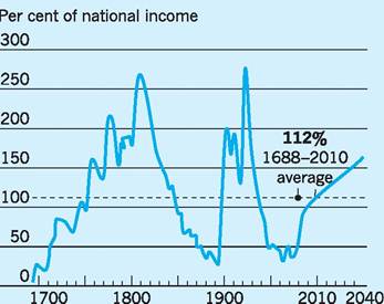
Fig. 18.3 UK public debt since the 17th century. Sources: IMF data (various); Goodhart (1999).
amounts of securities via quantitative easing (see Chapter 20), have caused a sharp upward revision in the National Debt to around 90% of National Income in 2010, with a projected rise to around 155% of National Income in 2040, were the same expenditure patterns to continue. This projected trajectory for the National Debt is widely considered unsustainable, and it would be ‘punished’ by the financial markets and credit rating agencies were it to materialize, with long-term interest rates rising well above current levels. Interestingly, in 2010 the budgetary problems of Ireland and its reduced credit rating meant that borrowing for five years or more cost the Irish government an extra 4% more than Germany should it borrow over the same time period.
Public spending by function
Table 18.2 provides data on various aspects of the UK’s public sector expenditure by function over the period 1999-2009, with the third column indicating the importance of public spending on each function over the decade to 2009. We can see that Social Protection, Health and Education together comprise a significant 64% of TME.
The second column traces the changes in public spending on these various functions during the decade as a percentage of GDP. Again, we see the rapid growth in expenditure on Health, Education and Economic Affairs (especially Transport) over the decade.Fiscal ‘rules'
In addition to its commitment to the Maastricht criteria for fiscal convergence, in 1998 the Labour government committed itself to the following two important ‘fiscal rules’.
1 The ‘golden rule’: over the economic cycle the government will only borrow to invest and will not borrow to fund current expenditure.
Table 18.2 Public sector expenditure on services by function, 1999-2009.
| Services by function | Expenditure as a % of TME 2009-10 | Annual real growth of expenditure (%) 1999-2009 |
| 1 General public services of which: | 8.0 | 1.3 |
| Public & common services | 2.1 | 3.7 |
| International services | 1.2 | 7.0 |
| Public debt services | 4.7 | - 0.1 |
| 2 Defence | 5.7 | 2.0 |
| 3 Public order and safety | 5.2 | 4.9 |
| 4 Economic affairs of which: | 6.8 | 6.7 |
| enterprise and economic development | 1.4 | 5.9 |
| science and technology | 0.5 | 10.0 |
| employment policies | 0.6 | -1.6 |
| agri/forestry and fishing | 0.9 | 1.3 |
| transport | 3.5 | 13.2 |
| 5 Environmental protection | 1.7 | 8.4 |
| 6 Housing and community amenities | 2.3 | 1.6 |
| 7 Health | 17.9 | 9.0 |
| 8 Recreation, culture and religion | 7.1 | 4.2 |
| 9 Education | 13.2 | 6.5 |
| 10 Social protection | 33.2 | 4.2 |
| Note: Percentages may not add up to 100 due to rounding. | ||
| Source: Modified from HM Treasury (2010) Public Expenditure Statistical Analyses, Tables 4.3 & 4.4. | ||
2 The ‘public debt rule’: the ratio of public debt to National Income will be held over the economic cycle at a ‘stable and prudent’ level.
In effect, the ‘golden rule’ was designed to ensure that current expenditure would be covered by current revenue (see Chapter 19) over the economic cycle. Put another way, any PSBR (now public sector net cash requirement) must be used only for investment purposes, with ‘investment’ defined as in the National Accounts.
The ‘public debt rule’ was rather less clear in that the phrase ‘stable and prudent’ was somewhat ambiguous. However, taken together with the ‘golden rule’ it essentially meant that, as an average over the economic cycle, the ratio of PSBR to National Income could not exceed the ratio of investment to National Income. Given that, historically, government investment has been no more than 2-3% of National Income, then clearly the PSBR as a percentage of National Income must be kept within strict bounds.
These rules were designed to keep government budgets/spending in check as the UK was also committed to the Maastricht criteria for fiscal convergence. These included a 3% target for the overall ratio of the Public Sector Net Cash Requirement (PSNCR) to GDP, and a 60% target for the ratio of public debt to GDP.
To meet the requirements of these fiscal rules, it was essential for the government to introduce systems and procedures to enable it to better manage the planning, monitoring and control of public expenditure.
I Planning, monitoring and control
Governments must seek to plan levels of public expenditure several years into the future, especially since any rise in public expenditure must be financed either by additional taxation or by increased borrowing. Governments must also develop and apply procedures to monitor and control public expenditure. All three elements are involved to some extent in the Public Expenditure Survey ‘rounds’, to which all the spending departments must submit on a regular and ongoing basis.
Public Expenditure Survey (PES)
Planning public expenditure for the next three years begins with the Public Expenditure Survey (PES). As part of this process, the spending departments discuss their spending proposals with the Public Expenditure Division of the Treasury, with all proposals expressed in cash terms. This PES ‘round’ usually takes place between April and September of each year, with the results of the PES announced at the end of November when the Chancellor presents his Budget statement to Parliament. To avoid any planning ‘surprises’ the major spending departments, such as the Department of Social Security, actually undergo two PES rounds each year, the second lasting from October to April.
Control Total (CT)
We have already noted the importance attached to the ‘golden rule’, which has resulted in the government paying less attention to monitoring and controlling cyclical components of expenditure, such as unemployment benefit and various types of income support. This has led to the government establishing a new Control Total (CT) for public expenditure, which covers around 85% of the value of spending included in TEM. An underlying objective of the CT is to help government focus on those items of expenditure which it can directly control and which are independent of cyclical fluctuations in the economy. As well as excluding unemployment benefit and income support, the CT also excludes central government gross debt interest (since borrowing and interest payments tend to rise during recession and fall during recovery).
Until 1992, the ministers in charge of the spending departments would seek to agree on spending limits for their departments in bilateral negotiations with the Chief Secretary to the Treasury. The agreed sums for each department would then be added together and announced in an ‘Autumn Statement’ on public spending plans.
Since 1993, however, the spending ministers have had to meet face-to-face in Cabinet in October or November to fight for a share of the already established overall value for the CT. Any extra given to one spending department must be funded at the expense of another spending department by reallocating the provisionally agreed CT. Clearly this procedure is intended to restrict the possibility of ‘upward drift’ in total public spending, which many critics claimed to have been a constant feature of the previous system of simply aggregating the outcomes of bilateral negotiations between spending departments and the Treasury.
Further, since 1993 we have had a unified Budget in March, in which both revenue raising and expenditure plans are discussed together. Prior to 1993, the spending totals were announced in the ‘Autumn Statement’ and the revenue-raising measures to finance them were announced some six months later in the March Budget. This separation of time between announcing planned expenditure and announcing methods for raising the tax revenue to fund that expenditure was seen as encouraging public expenditure growth, since the public would be less likely to associate any need for higher taxes in the March Budget with announcements of higher public expenditure in the previous autumn. To remedy this, since 1993 we have had a ‘unified’ Budget, with planned expenditure and planned tax revenue announced together, reinforcing the linkage between the two.
Forecasts
Since the expenditure plans for each department must cover three years, forecasts are needed for the future expenditures required to implement the agreed policies over this time period. The expenditure forecasts for each department are based on the work of both internal departmental experts (e.g. statisticians and economists) and external experts (e.g. members of the independent Government Actuaries Department). Further, the basic assumptions on which these forecasts rest include estimates of future changes in variables such as retail prices, average earnings, unemployment rates, economic growth, etc. To ensure that the various departmental forecasts rest on common assumptions, the Treasury provides the spending departments with projections of the data on expected values for all these variables over the next three years.
Agreement by the government on the future spending plans of a department (departmental expenditure limits - DEL) implies agreement on the policy proposals produced by that department over the next three years. Such policy proposals are usually generated by the Policy Group which resides within each department. Members of the Policy Group will seek to reflect the political priorities of both the government and the departmental ministers, as well as taking into account the representation of various pressure groups and any current research findings in the field. These policy proposals, once agreed, are then costed by a specialist group within the department containing statisticians and economists, and these costings will in turn provide the basis for the department expenditure forecasts.
An outline of the various processes involved in a PES has been provided by the Department for Work and Pensions, which is used here to illustrate a system common to most spending departments (Fig. 18.4).
The Department for Work and Pensions is the largest spending department and accounts for around 30% of planned public expenditure. Expenditure on Social Security benefits, such as the Retirement Pension, Housing Benefit and Child Benefit, accounts for 95% of the total Department for Work and Pensions bill. Social Security expenditure is almost entirely demand led, so estimating future expenditure requires projections as to how that demand is likely to change in the future. Factors influencing Social Security expenditure can usefully be grouped into four key headings.
1 Demographic. The size and the structure of the population are key variables here, for example an ageing population will reduce spending on Child Benefit, but increase spending on retirement pensions.
2 Economic. The projected levels of unemployment, earnings, prices and economic growth will affect the demand for various types of benefit and therefore the amount of benefit paid.
3 Social. Changes in family structures, for example the frequency of divorce and of lone parenthood, will affect benefit expenditures.
4 Policy. The introduction of new benefits, changes to entitlement, changes to benefit rates, etc. will all affect benefit expenditure.
The government is obliged to report the differences between forecast expenditure and actual out-turn for any given year; drawing attention to any discrepancies between what was planned to be spent and what was actually spent is seen as helping the process of monitoring and controlling public expenditure.
The planning, monitoring and control of public expenditure can therefore be seen to have undergone considerable change in recent years, with the underlying aim of curbing tendencies towards an upward
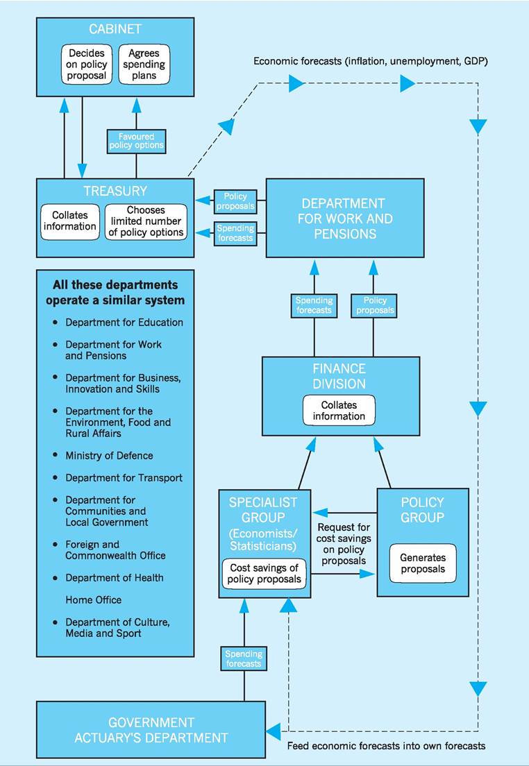
Fig. 18.4 The Public Expenditure Survey (PES) within the Department for Work and Pensions.
drift in spending totals. The procedures involved in the PES, the introduction of a new Control Total, the unified budget, obligations to report any discrepancies between forecast expenditures and actual out-turn are all parts of a more structured and accountable system for public expenditure.
A further element in such a system has been the so-called government drive for greater ‘efficiency’ in the public sector.
The drive for efficiency
Increasingly strident claims were made throughout the 1980s that, in the absence of competition, public services would always be produced inefficiently. One remedy might clearly be to increase such competition by privatizing the public services (see Chapter 8). Where this ‘remedy’ was not available then it was argued that efficiency could be improved by making sure that the delivery of public services conformed more closely to the needs of those who used them, rather than to the interests of those who provided them. This view led to a wave of reforms, including the introduction of contracting out and competitive tendering, the creation of Next Step Agencies, and the introduction of Value for Money Audits.
■ Contracting out and competitive tendering. Putting services previously provided through the public sector out to tender has led to cost savings of varying magnitudes. For example, there have been estimates of savings of 20% in the case of NHS catering and laundry, and savings of 14% in the case of highway services. In a number of other cases savings of 7% have been realized (Griffiths 1998).
■ Next Steps Agencies. These were introduced within government departments with the intention of improving the management of such departments. The idea here has been to separate the management of policy (the responsibility of central government) from operational management (the responsibility of the Agencies). For example, the Department for Work and Pensions has three main agencies, the Child Support Agency, JobCentre Plus and the Pensions, Disability and Carers Service. Such agencies have often been given the task of meeting a number of key performance indicators or targets, giving a yardstick against which their subsequent performance can be evaluated.
■ Value For Money (VFM) audits. These are part of the Financial Management Initiative (FMI) aimed at ensuring that public provision of goods and services is economic, efficient and effective. Under the FMI, central government departments have had to demonstrate to the Treasury that they have in place a VFM framework whereby audits are undertaken to check that managers are finding resource savings, while at the same time improving the quality of public services. Again, such procedures have often involved performance indicators.
■ Private Finance Initiative (PFI). The intention here has been to identify projects which can attract private sector finance to be used alongside public sector finance. The PFI is a method of providing funds for major capital investments where private companies are contracted to complete and manage the projects. The contracts (e.g. to build hospitals) are typically given to construction firms and the contract often lasts for up to 30 years. The contractors build the public services (hospitals) and they are then leased to the public and the government authority (e.g. Department of Health) who makes an annual payment to the private company. The total value of these forms of public-private partnerships in the UK currently amounted to some £68bn with future spending of £215bn due to be paid over the life of the contracts.
I The size of public expenditure
So far we have looked at changing shares within total public spending, but has the absolute level of public spending grown as fast as critics suggest? Such people usually point to a single statistic for evidence; for instance, that the public sector employs about 25% of the labour force or, as with Milton Friedman, that if public expenditure grows to around 60% of National Income then it will threaten to destroy freedom and democracy. Actually, estimates for the ratio of public spending to National Income vary widely, depending on the definitions used for each item. Figures for 2009/10 put total managed expenditure at around 46% of GDP at market prices (see Table 18.3). If, however, transfer payments are excluded from government expenditure, as they are from the measurement of National Income, then government
Table 18.3 Government spending as a proportion of National Income.
(a) Government spending as a proportion of GNP at factor cost (%)
| 1790 | 1890 | 1910 | 1932 1951 | 1966 | 1970 | 1976 |
| 12.0 | 8.0 | 12.0 | 29.0 40.2 | 40.2 | 42.2 | 48.7 |
| (b) Government spending as a proportion of GDP at market price (%) | ||||||
| 1978/79 | 1982/83 | 1986/87 | 1990/91 1992/93 1995/96 | 2000/01 | 2005/06 | 2009/10 |
| 45.1 | 48.1 | 43.6 | 39.4 43.7 41.8 | 36.8 | 41.3 | 46.2 |
Note: From 1977 onwards, an approximately 6% upward revision should be made to any government spending/National Income ratio if comparison with pre-1977 figures is to be made.
Sources: HM Treasury (2010) Public Expenditure Statistical Analyses; Brown and Jackson (1982).
expenditure falls dramatically to less than 30% of GDP at market prices. What, then, is the truth about the size of public expenditure?
An examination of data from the Office for National Statistics (ONS) suggests that as many as 10 measures could be used for estimating the size of public expenditure. The measure selected will depend on the question at issue. If the intention is to assess the financial resources passing through the hands of government, then a ratio involving TME might be appropriate. However, the ONS’s definition of National Income in the Blue Book excludes current grants and other transfers. Strictly, therefore, these same items should be excluded from government expenditure. They do not represent additional demand for resources; they are merely transfers of purchasing power from the taxpayer to other sectors of the community. Using this argument, a ratio of TME on goods and services of approximately 30% of National Income would appear to be the most appropriate measure.
No single measure of public expenditure has met with universal agreement, and even when one has been widely used for some time, it can be subject to change for a variety of reasons. In April 1977 the then widely used measure of general government expenditure was redefined to bring the UK into line with OECD accounting methods, and resulted in an apparent overnight reduction of some 6% in measured public expenditure. Again, what was previously tax relief may be reclassified as government expenditure, as with child tax allowances being replaced by Child Benefit in 1977. Public expenditure will also be affected by changes in the degree of ‘privatization’ (which is recorded as negative expenditure) or by changes in public sector pricing.
The National Income aggregate used for comparison will also influence our impression of the size of the public sector. Some ratios use domestic product, which measures resources produced entirely within the domestic circular flow. If, however, our interest was in the resources produced by UK nationals, wherever they happen to be located, then our ratio should use national product. Yet again, both domestic and national products could be valued ‘gross’ (including depreciation) or ‘net’ (excluding depreciation); at ‘market prices’, including the effects of taxes and subsidies, or at ‘factor cost’, excluding them.
For all these reasons, public spending ratios must be treated with caution when used in policy analysis.
Explanations of the growth in public expenditure
No matter what the definition, statistics show that the government sector of the economy has expanded over the last 150 years (see Fig. 18.5), both in money and real terms, and as a percentage of National Income. In Table 18.3, Brown and Jackson (1982), quoting a variety of sources, showed a dramatically rising trend of government spending as a proportion of GNP at factor cost up to 1976. The trend (using a different statistical series) continued upwards for data after 1976, reaching a peak of 48.1% in 1982/83. Between then and 2000 there has been a sustained fall
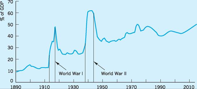
Fig. 18.5 General government expenditure as a percentage of GDP, 1890-2010 (projected).
in government spending as a percentage of National Income, though for a few years during the recession of the early 1990s the percentage had risen before resuming its downward path. Since 2000, and especially since the Comprehensive Spending Review of November 2002, there has been a renewed upward drift in government spending as a percentage of National Income, especially since the onset of the 2007 global recession. However, the 2010 Comprehensive Spending Review has made it clear that the future trend of general government expenditure as a percentage of GDP will be downwards over the coming years.
The explanation of the above trends and the difficulties involved in controlling public expenditure are based on two types of analysis: microeconomic and macroeconomic respectively.
Microeconomic analysis
Explanations based on microeconomic analysis suggest that additional public spending can be seen as the result of governments continually intervening to correct market failure. This would include the provision of ‘public goods’ such as collective defence, the police and local amenities (Cottrell 2002). An extra unit of such goods can be enjoyed by one person, without anyone else’s enjoyment being affected. In other words, the marginal social cost of provision is zero, and it is often argued in welfare economics that the ‘efficiency’ price should, therefore, be zero. Private markets are unable to cope with providing goods at zero price, so that public provision is the only alternative should this welfare argument be accepted. Microeconomic analysis would also cover extra public spending due to a change in the composition of the ‘market’, such as an ageing population incurring greater expenditure on health care.
Macroeconomic analysis
There are also explanations of the growth of public spending based on long-run macroeconomic theories and models. The starting point in this field is the work of Wagner (see Bird 1971), who used empirical evidence to support his argument that government expenditure would inevitably increase at a rate faster than the rise in national production. Wagner suggested that ‘the pressures of social progress’ would create tensions which could only be resolved by increased state activity in law and order, economic and social services, and participation in material production. Using the economists’ terms, Wagner was in effect suggesting that public-sector services and products are ‘normal’, with high income elasticities of demand. Early studies in the UK by Williamson during the 1960s tended to support Wagner, indicating overall income elasticities for public-sector services of 1.7, and for public-sector goods of 1.3, with similar results in other advanced industrialized countries.
Further evidence in favour of Wagner’s ideas came during the 1980s when studies by the OECD concluded that the proportion of GNP absorbed by public expenditure between 1954 and the early 1980s on ‘merit goods’ (education, health and housing) and ‘income maintenance’ (pensions, sickness, family and unemployment benefits) had doubled from 14% to 28%, as an average across all the advanced industrialized countries, with high income elasticities and low price elasticities playing a major part in this observed growth. Surveys of less developed economies were, however, more confusing, with econometric studies suggesting that little of the growth in public spending could be ‘explained’ by rising incomes (or low price elasticities).
Peacock and Wiseman’s ‘displacement theory’ (Peacock and Wiseman 1961), covering the period 1890-1953, suggested that public spending was not rising with the smooth, small changes predicted by Wagner, but that it was displaced (permanently) upwards by social upheavals associated, for instance, with depressions or wars leading to demands for new social expenditure (Fig. 18.5 above indicates the displacements of 1914-18 and 1939-45). Displacement theory has, however, been criticized for giving insufficient weight to political influences on the level of public expenditure. A further criticism of ‘displacement’ theory is the fact that for the UK there is little evidence that ratchet increases in public spending are long lasting. In fact, where the ratio of public expenditure to National Income continued to rise in the 1970s and 1980s, it was more easily explained by downward shifts of trend National Income in recession, with consequent increases in spending on unemployment benefits and social services, rather than through any upward revision of government expenditure plans.
The conclusion that must be drawn from reviewing such work is that there is no definite micro- or macro-explanation of the growth path for public expenditure. It then follows that there is no inevitable ‘law’ ensuring that public expenditure becomes a progressively rising proportion of National Income. However, in a recessionary period such as that of the early 1990s, increased spending on unemployment and social services may indeed cause a sharp increase in the share of public expenditure in National Income. The same result can be expected from explicit attempts by the UK government to raise the quality of public services and spending per head on those services to levels already reached within the EU economies (Griffiths 2002). Demographic changes may also conspire to raise the share of public expenditure. There has been considerable debate as to the mounting ‘burden’ on the working population likely to result from the growing number of pensioners in the next few decades. It has been estimated that the UK dependency ratio - the non-working population divided by the working population - will have risen from the current 0.52 to 0.62 by 2030. By 2030, therefore, each worker will be required to contribute 18% more real income to sustain the current level of welfare provision. It is scenarios such as this which have led to renewed scrutiny of the practicability of a welfare state along present lines.
I International comparisons
Given that public expenditure has grown over time in the UK, how do we compare with other countries? Conclusions based on OECD surveys indicate that UK public expenditure patterns are similar to those in most other advanced industrialized countries, although inferences drawn from international surveys must be treated with caution. The OECD definitions are frequently different from national ones, public sector boundaries vary between countries, and fluctuating exchange rates compromise any attempt at a standard unit of value.
Table 18.4 indicates that the growing share of UK public expenditure in National Income has been paralleled in other countries. If anything, public expenditure has grown less quickly in the UK, at least up to 2007. For example, in 1964 the UK was joint third highest, with Germany, of the 14 countries shown in Table 18.4, and by 1989 it was only eleventh highest of those same 14 countries. By 2005 it was still in eleventh place until the financial shock of the post 2007/08 period resulted in the UK rising to fifth highest in 2010. Compared to the average performance of Euro area countries, the UK’s government outlay as a percentage of GDP has remained below the Euro area average since 1979, only rising above it in 2010 with increased expenditures on stimulating the UK economy.
Table 18.4 Total outlays1 of government as a percentage of GDP at market prices: some international comparisons.
| 1964 | 1974 | 1979 | 1989 | 1999 | 20102 | |
| Australia | 22.1 | 31.6 | 31.4 | 33.1 | 34.4 | 34.8 |
| Austria | 32.1 | 41.9 | 48.9 | 50.0 | 53.7 | 51.9 |
| Belgium | 30.3 | 39.4 | 49.3 | 55.7 | 50.2 | 54.4 |
| Canada | 28.9 | 36.8 | 39.0 | 44.6 | 42.7 | 43.2 |
| Denmark | 24.8 | 45.9 | 53.2 | 59.4 | 55.5 | 60.1 |
| France | 34.6 | 39.3 | 45.0 | 49.4 | 52.6 | 55.9 |
| Italy | 30.1 | 37.9 | 45.5 | 51.5 | 48.2 | 51.6 |
| Japan | N/A | 24.5 | 31.6 | 31.5 | 38.6 | 40.8 |
| The Netherlands | 33.7 | 47.9 | 55.8 | 55.9 | 46.0 | 52.4 |
| Norway | 29.9 | 44.6 | 50.4 | 54.6 | 47.7 | 45.3 |
| Sweden | 31.1 | 48.1 | 60.7 | 59.9 | 58.6 | 56.0 |
| UK | 32.4 | 44.9 | 42.7 | 41.2 | 38.8 | 52.5 |
| USA | 27.5 | 32.2 | 31.7 | 36.1 | 34.2 | 41.6 |
| Germany | 32.4 | 44.6 | 47.6 | 45.5 | 48.2 | 47.9 |
| Euro area | 32.1 | 40.7 | 45.5 | 47.8 | 48.2 | 50.8 |
| Average OECD countries | 29.9 | 36.3 | 41.2 | 41.5 | 39.7 | 44.4 |
1Total government outlay = final consumption expenditure + interest on national debt + subsidies + social security transfers to households + gross capital formation.
2Projected.
Source: Adapted from OECD (2010) Economic Outlook, June, and earlier volumes.
Fiscal tightening
The financial crisis of 2007/08 precipitated a sharp recession in the UK economy which resulted in a serious fall in government revenues actually received in 2008/09 and revenues expected in subsequent years. This, combined with rapid increases in government spending to rescue financial institutions, support quantitative easing, provide improved services and pay benefits for higher unemployment, resulted in a rapid increase in the budget deficit, which rose as high as 11% of GDP in 2009/10 (see Fig. 18.2, p. 354). These growing fiscal deficits meant that the UK, as well as other major economies, had to ‘repair’ their public finances with a combination of expenditure reduction and taxation increases. The UK government has concentrated on the expenditure side of the equation to make these adjustments, with 70% of the projected ‘closure’ of the budget deficit by 2015 involving planned public expenditure cuts.
To place this ‘fiscal tightening’ in context it will be useful to provide a background to UK public expenditure issues and the various solutions suggested by both the last Labour government and the Conservative/ Liberal coalition government post-2010.
It can be seen (Table 18.5) that the tightening of the finances by both governments was mostly on the public expenditure side with over 70% stemming
Table 18.5 Composition of fiscal tightening to 201415: Labour and Coalition government estimates.
| March 2010 Budget (£bn) | June 2010 Budget (£bn) | |
| Tax | 21.5 | 29.8 |
| Spending | -50.9 | -82.8 |
| Investment spending | -17.2 | -19.3 |
| Current spending | -33.7 | -63.5 |
| of which | ||
| Debt interest | -7 | -10.0 |
| Benefits | -0.3 | -10.7 |
| Public services | -27.0 | -42.8 |
| Total fiscal tightening | 72.4 | 112.6 |
| Source: Crawford (2010). | ||
from expenditure cuts and around 30% from tax rises. The Coalition government’s plans announced in June 2010 involved a further ‘tightening’ (cuts in public expenditure/increases in taxation) from £72.4bn to £112.6bn by 2014/15. This was around 56% more than the fiscal tightening envisaged by the Labour government in March 2010. In June 2010 the Chancellor of the Exchequer announced that there would be two basic ‘rules’ to be followed.
■ Rule 1: that the forecast time horizon would be 2014/15 and that a fiscal tightening of 5.9% of GDP or £112.6bn would be required over that period.
■ Rule 2: that debt as a share of GDP should fall by the end of the forecast time horizon. The composition of the ‘tightening’ was further modified in October 2010 with a shift towards reducing spending on benefits by more than planned and reducing spending on public services by less than planned.
The aim of these policies is to bring the budget back to near balance by 2014/15. Whatever the ‘necessity’ of cutting public expenditure in the short to medium term in response to the global financial crisis, there is still the question relating to whether it is appropriate to restrict public expenditure as a general principle. It is to this question that we now turn.
Should public expenditure be restricted?
Freedom and choice
Arguments for controlling or reducing the size of public expenditure are wide-ranging but not always convincing.
One argument is that excessive government expenditure adversely affects individual freedom and choice. First, it is feared that it ‘spoonfeeds’ individuals, taking away the incentive for personal provision, as with private insurance for sickness or old age. Second, it is feared that by impeding the market mechanism it may restrict consumer choice. For instance, the state may provide goods and services that are in little demand, whilst discouraging others (via taxation) that might otherwise have been bought. Third, it has been suggested that government provision may encourage an unhelpful separation between payment and cost in the minds of consumers. With government provision, the good or service may be free or subsidized, so that the amount paid by the consumer will understate the true cost (higher taxes, etc.) of providing him or her with that good or service, thereby encouraging excessive consumption of the item.
Crowding out the private sector
Conservative governments have long believed that (excessive) public expenditure was at the heart of the UK’s economic difficulties. They regard the private sector as the source of wealth creation, part of which it saw as being used to subsidize the public sector. Sir Keith Joseph clarified this view during the 1970s by alleging that ‘a wealth-creating sector which accounts for one-third of the national product carries on its back a State subsidized sector which accounts for two-thirds. The rider is twice as heavy as the horse.’
Bacon and Eltis (1978) attempted to give substance to this view. They suggested that public expenditure growth had led to a transfer of productive resources from the private sector to a public sector producing largely non-marketed output, and that this had been a major factor in the UK’s poor performance in the post-war period. Bacon and Eltis noted that public-sector employment had increased by some 26%, from 5.8 million workers to 7.3 million, between 1960 and 1978, a time when total employment was largely unchanged. They then alleged that the private (marketed) sector was being squeezed by higher taxes to finance this growth in the public sector - the result being deindustrialization, low labour productivity, low economic growth and balance of payments problems (see also Chapter 19). The Bacon/ Eltis assumption that the public sector invariably ‘crowds out’ the private sector has been challenged from various directions. For example, research suggests that although growth in public expenditure and taxes seem to have some negative effects on overall productivity and growth in the short run, their long- run efforts are less predictable (Handler et al. 2005). The same research also concluded that government R&D expenditures do not crowd out private R&D activities and that additional public expenditure by smaller economies may be growth enhancing.
Control of money
Another argument used by those who favour restricting public expenditure is that it must be cut in order to limit the growth of money supply and to curb inflation. The argument is that a high PSBR - now known as the public sector net cash requirement - following public expenditure growth, must be funded by the issue of Treasury bills and government stocks. Since there are inadequate ‘real’ savings to be found in the non-bank private sector, these bills and bonds inevitably find their way into the hands of the banks. As we will see in Chapter 20, they may then form the basis for a multiple expansion of bank deposits (money), with perhaps inflationary consequences.
A related argument is that public expenditure must be restricted, to limit not only the supply of money but also its ‘price’ - the rate of interest. The suggestion here is that to sell the extra bills and bonds to fund a high PSBR, interest rates must rise to attract investors. This then puts pressure on private-sector borrowing, with the rise in interest rates inhibiting private-sector investment and investment-led growth. A major policy aim of the government has, therefore, been to reduce public-sector borrowing. However, a weakness with this argument is that is assumes that the supply of money in an economy is fixed. If the government increases its expenditure but at the same time increases the amount of money in the economy (see quantitative easing, Chapter 20, p. 419), it need not deprive the private sector of finance and interest rates will not be forced upwards.
Incentives to work, save and take risks
There are also worries that increased public spending not only pushes up government borrowing to fund a high PSBR, but also leads to higher taxes, thereby reducing the incentives to work, save and take risks. The evidence linking taxes to incentives is reviewed in Chapter 19. Suffice it to say here that the evidence to support the general proposition that higher taxes undermine the work ethic is largely inconclusive.
Balance of payments stability
A further line of attack has been that the growth of public expenditure may have destabilized the economy. During the 1970s and early 1980s this view was implied by the Cambridge Economic Policy Group (CEPG), who used an accounting identity (see Chapter 24) to demonstrate that a higher PSBR must lead to a deterioration in the balance of payments. The common sense of their argument is that higher public spending raises interest rates and attracts capital inflows, which in turn raise the demand for sterling and therefore the exchange rate. A higher pound then makes exports dearer and imports cheaper, so that the balance of payments deteriorates.
These various lines of reasoning have been challenged by, amongst others, the New Cambridge School which suggested that the relationships between the public sector and economic management may by no means be so simple. In fact, one adherent of the New Cambridge School, Lord Kaldor, went so far as to say that there was no empirical support for a high PSBR leading either to substantial growth in money supply or to high rates of interest. Similarly, the claim that resources liberated by the public sector would automatically find their way into the private sector was hardly supported by the rising unemployment trend of the early 1980s and early 1990s. Another criticism has pointed to the fact that public expenditure cuts, rather than helping to control unemployment (by cutting inflation in a monetarist model), have either caused or exaggerated current unemployment (see Chapter 23).
I Conclusion
The definition of public expenditure is by no means clear-cut and must depend upon the question at issue. Since National Income also has many variants, any public expenditure/National Income ratio must be treated with caution. Whatever the definition chosen, the proportion of government spending in National Income rose steadily throughout the twentieth century. The reduction in the growth of National Income played an important part in raising the ratio in the early 1980s, early 1990s and since 2007, both directly, by restricting the denominator, and indirectly, by causing unplanned increases in expenditure on social security. Whether a growing public sector ‘crowds out’ or otherwise adversely affects the private sector is a matter of deep controversy. Certainly in comparative terms the UK is by no means exceptional, with the share of UK government spending in National Income well below the average for the EU countries. More ‘rigour’ has been imposed on procedures to plan, monitor and control public expenditure. This, together with renewed growth in National Income, helped to progressively reduce the ratio of government spending to National Income to around 37% in 2000, though the renewed emphasis on increased government spending since then has seen government spending at around 47% of National Income in 2010.
The move, in late 1992, towards a new ‘control total’ for public spending made it clear that the government would continue to seek a tight fiscal stance, especially on items of expenditure of a non-cyclical nature. The determination of the government to adhere to the Maastricht criteria of a ratio of PSBR to GDP below 3%, and of public debt to GDP below 60%, suggests that public expenditure will remain closely controlled. This view was further strengthened by the announcement of fiscal ‘rules’ in 1998, especially the ‘golden rule’ whereby government borrowing would only be undertaken to support public investment and not current consumption. The intention of the Coalition government is to eliminate the budget deficit by 2015, manly by restricting the growth of public expenditure.
Key points
■ Although government spending rose in real terms by around 1% per annum between 1990 and 2000, this was less than the growth in real National Income.
■ As a result the share of government spending in National Income fell from almost 45% in 1992/93 to around 37% in 2000/01.
■ Successive government spending reviews since 2000 have resulted in substantial real-term increases in government spending, which accounted for around 47% of National Income by 2009/10.
■ Critics argue that too high a proportion of government spending goes on ‘rescue’ and ‘welfare’ and too little on ‘renewal’. In this view more of the public purse should be used to support ‘investment’ type expenditures (on human or physical capital) directed towards raising future National Income.
■ Total Managed Expenditure (TME) has now replaced general government expenditure (GGE).
■ International comparisons do not suggest that UK public expenditure is exceptionally high as a percentage of GDP. In 2010 it was only 5th highest out of 14 countries investigated, and only marginally above the Euro area average.
■ Many of the reasons put forward for controlling public expenditure involve the desire to cut the PSBR (now the public sector net cash requirement). The government concern is that too high a PSBR will force higher taxes and interest rates, with adverse effects on incentives and investment in the private sector.
■ Part of the ‘convergence criteria’ within the EU involves keeping the PSBR no higher than 3% of GDP, implying tight control of public expenditure, keeping to this criterion has been difficult since the financial crisis of 2007/08.
■ The ‘fiscal rules’ of the last government have been replaced by the Conservative/ Liberal coalition’s two broad rules. The intention is to close the budget deficit from the 11% of GDP of 2010 to around zero by 2015.
■ The procedures for planning, monitoring and controlling public expenditure have been modified. These include changes to the departmental PES, a new ‘Control Total’, a unified Budget, relating spending forecasts to out-turns, and various initiatives to increase efficiency in the public sector.
Now try the self-check questions for this chapter on the Companion Website. You will also find useful links to relevant websites.
References and further reading
Bacon, R. and Eltis, W. (1978) Britain’s Economic Problem: too few producers (2nd edn), Basingstoke, Macmillan.
Beachill, R., Spoor, C. and Wetherly, P. (2002) Keeping the economy healthy, Economic Review, 20(2): 2-5.
Benassy-Quere, A. and Coeure, B. (2010) Economic Policy, Oxford, Oxford University Press.
Bird, R. M. (1971) Wagner’s law of expanding state activity, Public Finance, 26(1): 1-26.
Brown, C. V. and Jackson, P. M. (1982) Public Sector Economics (2nd edn), London, Martin Robertson.
Cottrell, D. (2002) Public goods: an insoluble economic problem?, Economic Review, 20(1), September.
Crawford, R. (2010) ‘Where the axe fell’, IFS Spending Review 2010, Briefing Paper, London, Institute for Fiscal Studies.
Department of Trade and Industry (2006) The Government’s Expenditure Plans 2006-07 to 2007-08, London, The Stationery Office.
Flemming, J. and Oppenheimer, P. (1996) Are government spending and taxes too high (or too low)?, National Institute Economic Review, July, 58-73.
Giavazzi, F. and Blanchard, O. (2010) Macroeconomics: A European Perspective, Harlow, Financial Times/Prentice Hall. Goodhart, C. (1999) Monetary policy and debt management in the UK, in Chrystal, K. Alec (ed.), Government Debt Structure and Monetary Conditions. London, Bank of England.
Griffiths, M. A. (1998) Government expenditure and efficiency, Money Management Review, 51: 10-13.
Griffiths, A. (2002) The Budget and the Comprehensive Spending Review 2002, British Economy Survey, 32(1): 17-21.
Handler, H., Knabe, B., Koebel, M., Schratzenstaller, M. and Wehke, S. (2005) The Impact of Public Budgets on Overall Productivity, WIFO Working Paper no. 255, Vienna, Austrian Institute of Economic Research. HM Treasury (2010) Public Expenditure Statistical Analyses 2010, London.
Joseph, K. (1976) Monetarism is not Enough, London, Barry Rose.
OECD (2010) Economic Outlook, June, Paris, Organisation for Economic Cooperation and Development.
Papava, V. (1993) A new view of the economic ability of the government; egalitarian goods and GNP, International Journal of Social Economics, 20(8): 56-62.
Peacock, A. and Wiseman, J. (1961) The Growth of Public Expenditure in the United Kingdom, Manchester, UMI.
Rowthorn, R. (1992) Government spending and taxation in the Thatcher era, in Michie, J. (ed), The Economic Legacy, 1979-1992, London, Academic Press.
Weir, J. (1998) Government spending: a view from the inside, Money Management Review, 51: 5-7.
Wolf, M. (2010) UK public debt since the 17th century, Financial Times, 3 November.