The Dominance Approach

The dominance approach provides a framework to ascertain whether unambiguous poverty comparisons can be made across a whole class or range of poverty measures and parameter values.

The dominance approach has been widely used in the measurement and analysis of poverty and also of inequality within a unidimensional framework (Atkinson 1970, 1987; Foster and Shorrocks 1988a,b; Jenkins and Lambert 1998). It was extended to the multidimensional framework for inequality measurement by Atkinson and Bourguignon (1982, 1987) and Bourguignon (1989), then to the context of multidimensional poverty measurement by Duclos, Sahn, and Younger (2006a) and Bourguignon and Chakravarty (2009). We first elaborate the dominance approach in the unidimensional context and then show how it has been extended to the multidimensional context.

3.2.3 POVERTY DOMINANCE IN UNIDIMENSIONAL FRAMEWORK

In the unidimensional context, a society is judged to ‘poverty dominate' another society with respect to a particular poverty measure if the former has equal or lower poverty than the other society for all poverty lines and strictly lower poverty for at least some poverty lines.

In poverty measurement, the tool most frequently used for dominance analysis is stochastic dominance. Stochastic dominance has different orders: first, second, and higher, which can be presented in terms of univariate cumulative distribution functions (CDF). The two achievement vectors x and y presented in the previous paragraph may also be represented by using CDFs F_x and F_y, respectively. Thus, vectors x and y can also be referred to as distribution x and y, respectively. The value of CDF F_x at any achievement level b ∈ R₊, denoted by F_x(b), is the share of population in distribution x with achievement levels less than b. Similarly, F_y(b) denotes the share of the population in distribution y with achievement levels less than b.

We first introduce the concept of first-order stochastic dominance for a unidimensional distribution.^[86] Distribution x first-order stochastically dominates distribution y, which

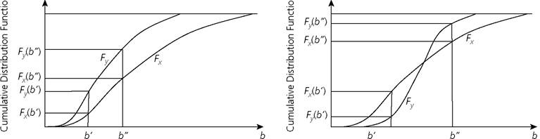
Figure 3.4. First-order stochastic dominance using cumulative distribution functions

is written x FSDy, if and only if F_x (b) ≤ F_y(b) for all b and F_x (b) < F_y (b) for some b.^[87] In other words, the CDF of x lies to the right of the CDF of y.

The value of a CDF corresponding to a certain level of achievement is the proportion of the population with achievements below that level. Interestingly, if a particular level of achievement is set as a unidimensional poverty line (b' = z_u), then the value of the CDF at z_u is the headcount ratio P₀ (see section 2.1). Thus, F_x (z_u) and F_y (z_u) are the headcount ratios for distributions x and y for poverty line z_u, respect­ively. Then, x FSD y if and only if P₀ (x; z_u) < P₀ (y; z_u). In other words, first-order stochastic dominance is equivalent to the condition when the headcount ratio in distribution x is either equal to or lower than that in distribution y for all poverty cutoffs. Equivalently, y has no lower headcount ratio than x for all poverty cutoffs. Moreover, first-order stochastic dominance provides results beyond the headcount ratio. As Atkinson (1987) shows, if one distribution first-order stochastically dominates another distribution, then poverty is equal or lower in the former distribution for all poverty measures (and any monotonic transformation of these measures) satis­fying population subgroup decomposability and weak monotonicity. The result, as Atkinson discusses, can be extended to measures that are not necessarily subgroup decomposable.

Unlike Panel I, Panel II shows a situation where the CDFs cross each other. For all b to the left of the crossing, F_x (b) > F_y(b), whereas for all b to the right of the crossing, F_x (b) < F_y(b).

3.2.4 POVERTY DOMINANCE IN THE MULTIDIMENSIONAL FRAMEWORK

This approach has been extended to the multidimensional context by Duclos, Sahn, and Younger (2006a) and Bourguignon and Chakravarty (2009). Poverty dominance in the multidimensional framework is slightly different in that it needs to consider the identification method as well as the assumed relationship between achievements, namely, whether they are considered substitutes, complements, or independent. As discussed in Chapter 2, the identification of those who are multidimensionally poor is not as straightforward as in the unidimensional framework. In a multidimensional dominance approach, a poverty frontier based on an overall achievement value of well-being for each individual is used for identification, and the overall achievement is required to be non-decreasing in each dimensional achievement. The poverty frontier belongs to the so-called aggregate achievement approach (section 2.2.2) and it is defined as the different combinations of the d achievements that provide the same overall achievement as an aggregate poverty line or subsistence level of well-being.

The poverty frontier method—like other identification methods such as counting— encompasses the two extreme criteria for identification, namely, union and intersec­tion, as well as intermediate cases. The poverty frontier method for identification is presented in Figure 3.5 using two dimensions. The horizontal axis of the diagram represents achievements in dimension 1, and the vertical axis denotes achievements in dimension 2. The deprivation cutoffs of both dimensions are denoted by z₁ and z₂, respectively. The intersection frontier is given by the bold black line, and any person with achievement combinations to the left of and below this line is identified as poor. Similarly, the union frontier is given by the dotted line, and any person with achievement combinations to the left of or below the dotted line is considered poor.

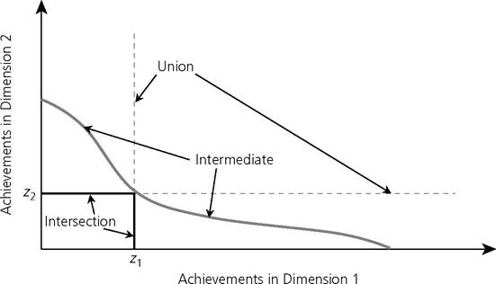
Figure 3.5. Identification using poverty frontiers

Finally, an example of an intermediate criterion is given by the bold grey line, and any person with an achievement combination falling below this frontier is identified as poor.

Poverty dominance is defined by Duclos, Sahn, and Younger (2006a) in the multidi­mensional context as follows. Once a poverty frontier is selected for identifying the poor, for any two societies with achievement matrices X, Y ∈ X, the society with achievement matrix X poverty dominates the society with achievement matrix Y for poverty measure P, which we refer to as XPY, if and only if P (X; z) ≤ P(Y; z) for all z ∈ z and P (X; z) < P(Y;z) for some z ∈ z.

As in the unidimensional framework, the achievement matrices presented in the previous paragraph may also be represented using joint CDFs F_x and F_y, respectively.^[89] Each column of an achievement matrix can be represented by a univariate marginal distribution.

How overall multidimensional poverty is sensitive to association between dimensions depends on the relation between dimensions as discussed in section 2.5.2. If dimensions are seen as substitutes, then an increase in association between dimensions, with the same set of marginal distributions, should not reduce overall poverty. On the contrary, if dimensions are complements, then an increase in association between dimensions, with the same set of marginal distributions, should not increase poverty. Duclos, Sahn, and Younger (2006a) present the stochastic dominance results for two dimensions, assuming the dimensions are substitutes. Thus, they show under the assumption of substitutability that if the joint cumulative distribution function Y lies above the joint cumulative distribution X or F_y (b₁, b₂ j > F_x(b₁, b₂) for all b₁ b₂ ∈ K₊, then XPY for all poverty measures that satisfy weak monotonicity and subgroup decomposability and use either union, intersection, or any intermediate poverty frontier method for identification. Note that the condition F_y (b₁, b₂) > F_x(b₁, b₂) for all b₁ b₂ ∈,R₊ is an intersection-like condition because F_y (b₁, b₂) and F_x (b₁, b₂) denote the shares of population with achievements less than b₁ in dimension 1 and at the same time achievements less than b₂ in dimension 2. This is analogous to the rectangular area bounded by the black bold lines in Figure 3.5. Thus, the novelty of this finding is that one should only check the intersection-like condition. For higher-order stochastic dominance conditions, readers are referred to Duclos, Sahn, and Younger (2006a).^[90]

Bourguignon and Chakravarty (2009) develop related first-order dominance condi­tions for multidimensional poverty measurement in the two-dimension case. Unlike Duclos, Sahn, and Younger, they use a counting approach for identification. They show that for poverty measures that satisfy deprivation focus, symmetry, replica­tion invariance, population subgroup decomposability, weak monotonicity, and weak deprivation rearrangement (substitutes), poverty dominance is required with respect to each marginal distribution and with respect to the joint distribution in the inter­section area (the rectangular area bounded by solid bold lines in Figure 3.5). This result is consistent with Duclos, Sahn, and Younger (2006a). Additionally, Bour- guignon and Chakravarty (2009) show that for poverty measures that satisfy the same previously mentioned properties but also converse weak deprivation rearrange­ment (complements), poverty dominance is required with respect to each marginal distribution and with respect to the joint distribution in the union area (L-shaped area bounded by the dotted lines in Figure 3.5). For a detailed discussion, see Atkinson (2003).

3.2.5 APPLICATIONS OF THE MULTIDIMENSIONAL DOMINANCE APPROACH

The Duclos, Sahn, and Younger (2006a) framework has been applied in several empirical studies. Batana and Duclos (2010) used the technique with two dimensions to compare multidimensional poverty across six members of the West African Economic and Monetary Union: Benin, Burkina Faso, Cote d'Ivoire, Mali, Niger, and Togo. The comparison of these six countries involved fifteen pairwise comparisons, and identified a statistically significant dominance relation for twelve of the pairwise comparisons. Anaka and Kobus (2012) employed the technique, also using two dimensions, to compare multidimensional poverty across Polish gminas or municipalities. Labar and Bresson (2011) used this approach to study the change in multidimensional poverty in China between 1991 and 2006 and showed that the change in multidimensional poverty was not unambiguous. Grab and Grimm (2011) extended this multidimensional dominance framework to the multi-period context and illustrated their approach using data for Indonesia and Peru.

Other applications of dominance analysis have also been undertaken recently. For example, Duclos and Echevin (2011) used a dominance approach to find that welfare in both Canada and the United States did not unambiguously change in terms of the joint distribution of income and health. In fact, although dominance in terms of income was prominent across the entire population, dominance across incomes did not hold across each health status. Extending the Atkinson and Bourguignon (1982) framework using four dimensions in the Indian context, Gravel and Mukhopadhyay (2010) found a robust reduction in multidimensional poverty between 1987 and 2002. The study used municipality-level information for three dimensions, not household-level information.

The above studies assume that the dimensions are continuous. In practice, most relevant indicators are discrete. Duclos, Sahn, and Younger (2006b) extend their multidimensional robustness approach to situations where one dimension is continuous but the rest of the dimensions may be discrete (Batana and Duclos 2011). For an alternative approach to discrete variables extending the Atkinson and Bourguignon (1982) framework, see Yalonetzky (2009, 2013).

3.2.6 Acriticalevaluation

The strength of the dominance approach is that when poverty dominance holds between a pair, then the comparison is unambiguous. No alternative specifications can alter the direction of comparison. Thus, it offers a tool to produce strong empirical assertions about poverty comparisons—assertions that hold across a range of poverty measures and in spite of any ‘controversial' decisions on parameter values. Even if distributions cross, and thus it is not possible to have a rank, it is possible to check where the crossing has taken place and identify limited areas of dominance, which can provide important information. In addition, the dominance approach takes into account the joint distribu­tion of achievements when identifying the poor and making poverty comparisons. The dominance approach has been used with both discrete and continuous data.

Despite its strengths, this approach has certain limitations that prevent it from being more widely used for empirical analysis. First, when dominance holds, conclusions about comparisons can be made, but when there is no dominance, no unambiguous comparisons can be made. In other words, the dominance approach can only provide a partial ordering—similar to Lorenz dominance in inequality measurement. Second, even in situations in which dominance comparisons are empirically possible and generate ordinal rankings of regions or societies across time, it is not possible to compare the extent of differences in poverty across two populations in any cardinally meaningful way. In other words, it is not possible to say how poor a region is compared to another or how much poverty has fallen or gone up over a certain period of time. The complete orderings and meaningful cardinal comparisons achieved using other methods, such as axiomatic measures, can be criticized as imposing arbitrariness or ‘creating artificial problems' (Sen 1997:5). However, it must also be recognized that the inability to offer a complete ranking in certain cases can make this tool of limited use from a policy perspective.

A third limitation of this approach (although not exclusive to it) is that the dominance conditions depend on assumptions regarding the relationship between achievements (either substitutes or complements). In practice, all empirical applications so far have assumed substitutability between achievements because conditions and their statistical tests in this case are more fully developed. As Duclos, Sahn, and Younger (2006a) point out, one of the reasons for not pursuing the case of complementarity further is that it would drastically limit the scope of robust orderings across alternative poverty frontiers. Furthermore, the test developed by Duclos, Sahn, and Younger (2006a) is more suitable for measures that use the aggregate achievement approach (poverty frontier) to identification than for measures that use a counting approach.

Fourth, although in this section we present the results in terms of population, it may be empirically challenging to compute dominance using more than two or three dimensions due to the ‘curse of dimensionality'—the need for the sample size to increase exponentially with the number of dimensions. As Duclos, Sahn, and Younger (2006a) put it, ‘in theory, extending our results to more than two dimensions is straightforward. In practice, though, most existing datasets in developing countries are probably not large enough to support tests on more than a few dimensions of wellbeing. This is because [of] the curse of dimensionality...' (p. 944). In such cases of higher dimensionality, other tests or procedures may be required.^[91] Another relevant point for the empirical implementation of the dominance approach is that there is often noise at the extremes of the distribution that one may wish to ignore, because otherwise results maybe artificially biased. For this reason, one may want to base the dominance criteria on a range that starts, for example, at certain percentage of the median of the distribution of each variable.

Finally, in the multidimensional context, dominance results beyond first order require more stringent conditions on the individual poverty function, such as those on signs of third order, fourth order, derivatives, and cross-derivatives, which are less intuitive (see Duclos, Sahn, and Younger 2006a and Atkinson 2003).

The remaining three sections present methodologies that create indices of multidi­mensional poverty reflecting the joint distribution across dimensions. As in the case of Venn diagrams and the dominance approach, each approach requires that information be available for the same unit of analysis so that the joint distribution among dimensions can be captured. We first outline some of the widely applied multivariate statistical techniques used in the analysis and measurement of multidimensional poverty and well-being.

3.3