Statistical Approaches

Statistical techniques are widely used in the design of poverty measures as well as in measures of well-being (Nardo et al. 2008; Maggino and Zumbo 2012). Key techniques include principle component analysis, multiple correspondence analysis, cluster analysis, latent class analysis, and factor analysis.

We divide the statistical techniques into two categories. Figure 3.6 sketches this classification. The two categories are: descriptive methods, whose primary aim is to describe a multivariate dataset, and model-based methods, which additionally attempt to make inferences about the population (Bartholomew et al. 2008). One of the challenges in surveying statistical approaches is that applied methodologies vary widely, but our classification does summarize the methods most frequently used.^[92]

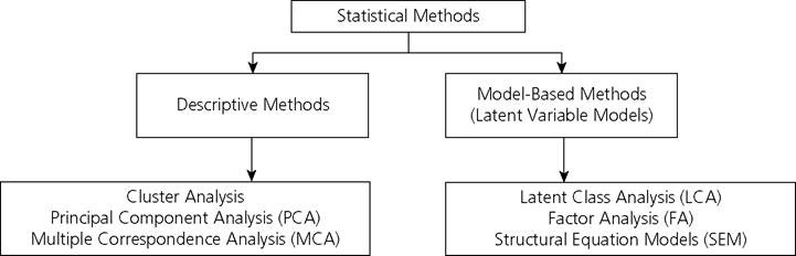
Figure 3.6.

As depicted in Figure 3.6, descriptive methods comprise cluster analysis, principal component analysis (PCA), and multiple correspondence analysis (MCA). The main difference between PCA and MCA is the scale of variables used. PCA is used when variables are of cardinal scale, while MCA is appropriate when variables are categorical or binary.^[93] The model-based methods are latent variable models and cover latent class analysis (LCA), factor analysis (FA), and, more generally, structural equation models (SEM).^[94] This section illustrates the use of PCA, MCA, and FA for aggregating dimensional achievements or deprivations for each person. These aggregated values may subsequently be used to identify the poor and to create poverty indices. We also illustrate cluster analysis and LCA as methods for grouping similar individuals or households together, which can be understood as a form of identification of the poor.

3.3.1 SUB-STEPS IN AGGREGATION WITHIN MULTIVARIATE STATISTICAL METHODS

The process of constructing a poverty index for a population has different sub-stages. Often these sub-stages of aggregation do not receive enough attention in the literature covering composite indices built using statistical methods, as the primary goal is to obtain a final aggregate number. In contrast, this section follows and makes explicit every single step followed in each of these techniques and itemizes the decisions made at each step. For different decisions taken, at each stage, different conclusions may arise. This novel

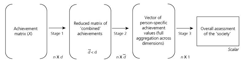
Figure 3.7. Aggregation sub-steps within multivariate statistical methods

presentation will enable readers to transparently compare poverty measures built using statistical methods with other approaches such as counting-based methods.

For example, when PCA or MCA is used, one needs to determine the number of components or axes to retain.

To provide an overview of statistical methods, we distinguish three sub-stages that may be used when generating summary measures of poverty (Figure 3.7). While these techniques are used for both well-being and deprivation analyses, here they are presented for deprivation analysis.

The aggregation sequence begins with a multivariate achievement matrix (X) as defined in Chapter 2, where the joint distribution of n persons across d indicators is often represented by second-order moments such as the correlation/covariance matrix (in the case of cardinal variables) or the multi-way contingency table (in the case of categorical variables) across the d indicators.^[95] Using these second-order moments of the joint distribution in the first stage of aggregation, one applies a multivariate method (say, PCA, MCA, or FA) that combines the d indicators into a smaller number of d (< d) new variables.

In PCA and MCA, one seeks to replace the original set of d indicators with a smaller number of d variables that account for most of the information in the original set, which

in PCA are uncorrelated or orthogonal.

The second stage of aggregation uses the reduced achievement matrix of size n ? d and combines the d variables, either by applying a multivariate method or an ad hoc procedure, to create a vector of size n ? 1 that represents the aggregate achievement values for each of the n persons. As a special case, if there is only one d and if there is no further aggregation, then d itself gives an overall measure of achievement for each person. An example of the two aggregation steps described above is followed by Ballon and Krishnakumar (2011). They first implement a so-called first-order factor model, where the d indicators are assumed to be manifestations of d latent or unobserved variables using confirmatory factor analysis in the form of a structural equation model.^[96] Then, they suggest using a so-called second-order factor model that combines these d variables into an ‘overall' factor, assuming that these d variables are also manifestations of a latent variable.^[97] The overall factor score for each person in this case is analogous to the aggregate achievement value in the aggregate achievement approach to identification described in section 2.2.2.

Alternatively, rather than using a multivariate method, one may use an ad hoc procedure—a common one being to combine the d variables using some form of weighted average. For example, in their study of quality of life among forty-three countries, Rahman et al. (2011) use the proportion of the total variance accounted for each component as its weight. Krishnakumar and Ballon (2008), in their estimation of children's capabilities in Bolivia, use the inverse of the factor's variance as its weight. However, other functional forms of weights could be envisaged. Note that the choice of weights may affect the cardinal interpretation of the results but not the ordinal one if the chosen weights preserve the order of the distribution of the factor scores as in the case of Krishnakumar and Ballon (2008).

The third stage aggregates the person-specific aggregate achievement values of all persons into an index that reflects the overall poverty of the population. Clearly, to achieve such a poverty index, identification of the poor needs to take place, comparing the person-specific aggregate achievement value against some poverty cutoff. This cutoff may be absolute but typically is relative in these methods. Thus, in this third stage, the n ? 1 vector, containing person-specific achievements, is compressed into a scalar measure to assess poverty in the society. Section 3.4.2 presents a brief overview of implementations of the various statistical approaches.

3.4.2 APPLICATIONS OF STATISTICAL APPROACHES IN POVERTY AGGREGATION

Filmer and Pritchett (1999, 2001) applied PCA to a set of asset variables found in the Demographic and Health Surveys and retained the first principal component in order to construct a household asset index. The asset index scores were standardized in relation to a standard normal distribution with a mean of 0 and a standard deviation of 1. All individuals in each household were assigned the household's standardized asset index score, and all individuals in the sample population were ranked according to that score.

Within the correspondence analysis literature, we find applications by Asselin and Anh (2008), Booysen et al. (2008), Deutsch, Silber, and Verme (2012), Batana and Duclos (2010), and Ballon and Duclos (2014). Asselin and Anh (2008) built an MCA composite index of human and physical assets to study poverty dynamics in Vietnam between 1999 and 2002. Booysen et al. (2008) applied MCA to obtain an asset index for comparing poverty over time and across seven West African countries. Deutsch, Silber, and Verme (2012) use correspondence analysis to analyse social exclusion in Macedonia. Batana and Duclos (2010) calculated a multidimensional index of wealth (ownership of durable goods and access to services) using MCA for a series of sub-Saharan African countries. This index was used to compare cross-country multidimensional poverty via sequential stochastic dominance analysis. Ballon and Duclos (2014) applied MCA to obtain two sets of values reflecting households' access to ‘public' assets (basic services) and ‘private' assets (durable goods) in Sudan and South Sudan. These two sets of MCA values were further used for measuring multidimensional poverty according to the Alkire and Foster (2011a) methodology.

Interesting applications of statistical techniques up to the last stage of aggregation (i.e. obtaining an overall well-being or deprivation index for the society) include those used by Kuklys (2005), Klasen (2000), and Ballon and Krishnakumar (2011). Kuklys used the factor scores obtained from a structural equation model as the input distributions in FGT poverty-type measures (Foster, Greer, and Thorbecke 1984). Ballon and Krishnakumar (2011) proposed an index of capability deprivation, where the input variables were the factor scores of a structural equation model that estimated children's capabilities. Klasen (2000) derived a material deprivation index for households in South Africa. Other interesting applications of structural equation models in development studies, although not focused on aggregation into a scalar measure, are the ones proposed by Di Tommaso (2007) for India, Wagle (2008) for Nepal and the United States, and Ballon (2011) for Cambodia.

3.4.3 A BRIEF AND FORMAL OUTLINE OF DIFFERENT STATISTICAL APPROACHES

This section presents in greater detail the three methods most commonly implemented for both identification and aggregation, namely, PCA, MCA, and FA. Additional methodological variations are also implemented; this section covers the more standard approaches.

3.4.3.1 Principal ComponentAnalysis

Principal component analysis was first proposed by Pearson (1901) and was further developed by Hotelling (1933). Hotelling derived principal components using mathem­atical arguments, leading to the standard algebraic derivation that optimizes the variance of the original dataset (known as an ‘eigen decomposition'), while Pearson approached PCA geometrically.^[98]

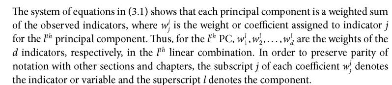
The main aim of PCA is parsimony.^[99] Basically, in PCA the d indicator variables are transformed into linear combinations called principal components. In this search for parsimony, one seeks to find fewer principal components (PCs) that retain most of the information in the original set of observed indicators. The information retained by the PCs is measured by the proportion of the total (sample) variance that is accounted for in each of the PCs. There is usually a trade-off between a gain in parsimony and a loss of information. If the original indicators are correlated, and especially if they are highly correlated, then one can replace them by a relatively small set of PCs—say, d, where d is smaller than d. If the original indicators are only slightly correlated, the resulting PCs will largely reflect the original set without much gain in parsimony. Clearly, the full set of PCs will fully account for the total variance of the original indicators and will be the case where no reduction in dimensionality is achieved. A particular feature of PCs is that these are uncorrelated (orthogonal).

Let us denote each PC by f^PC. In order to retain comparability with notation in other sections and chapters of this book, we denote the n ? d-dimensional achievement matrix by X, where d is the number of observed indicators, n is the number of persons, and x_ij is the achievement of person i in dimension j for all i = 1,..., n and j = 1,..., d. We denote the j^th observed indicator by XjTh For a given person i, the full set of PCs is a system of d linear combinations of these observed indicators.

This is written as

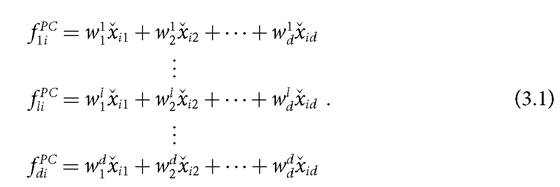
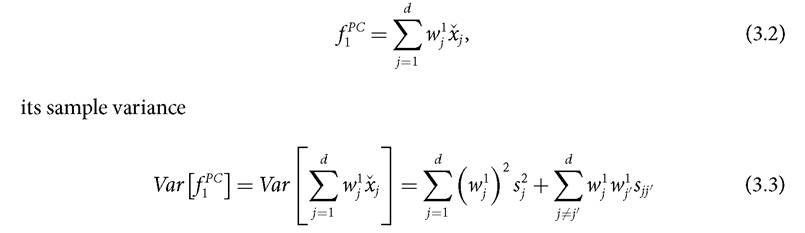
Our aim in poverty analysis is to replace the set of d observed indicators with a much smaller number of ‘transformed variables', here the PCs, that retain most of the information in the indicators, which is measured by the proportion of the total variance accounted for by each PC (Bartholomew et al. 2008: ch. 5). To obtain each PC, one requires an estimate of the weights (w∣) and of the variance of the PCs. These are obtained using the maximum variance properties. For a given sample, the maximum variance property of PCA defines the first principal component as the linear combination with maximal sample variance among all linear combinations of the indicators, so that it accounts for the largest proportion of the total sample variance (Rencher 2002). To achieve a maximum, one needs to add some normalization constraints on the coefficients

^[1] Note that in section 3.4.3 we formalize the use of statisitcal approaches using sample moments instead of population moments. For this reason, we use X _ij instead of X_ij, to denote the observed achievement of person i in dimension j.

^[1] This restriction ensures that weights are non-negative and each weight is bounded above by one.

^[1] For definitions of eigenvalues, eigenvectors, and singular value decomposition, see the statistical appendix A.6 of Mardia, Kent, and Bibby (1979).

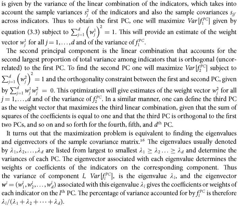
When the units of measurements across (cardinal) indicators vary or when the variances²⁷ across them differ widely, one may wish to use the sample correlation matrix R instead of the sample covariance matrix S. This is equivalent to standardizing each of the d indicators to have a mean of 0 and variance of 1, then finding the PCs of the standardized covariance matrix R. The principal components obtained from R will contribute evenly to total variation and thus be more interpretable. However, the components extracted from S, the unstandardized covariance matrix, will differ from those extracted from the correlation matrix²⁸ R, and so the percentage of variance accounted for by the components of each of the matrices will be different. Thus the decision to use either R or S may affect the final results.

Once one has computed the PCs and obtained an estimate of the weights and the variances of each PC, one needs to decide the number of components to retain. This is especially important in studies of deprivation that use PCA as the basis for obtaining either a person-specific or a society measure of poverty, as the results may vary depending on the number of PCs retained. This aspect has been thoroughly examined by Coste et al. (2005) while obtaining synthetic measures of deprivation in health.

There is a multiplicity of rules for determining the number of components to retain (Jolliffe 2002). The main guidelines for selecting components in PCA are based on a combination of the percentage of variance accounted for as in (3.3), the scree plot,²⁹ and the useful interpretation that the retained components may provide for analysis (Rencher 2002; Bartholomew et al. 2008). Following the first criterion, one will retain the first l components which account for a large proportion of total variation, say 70-80%. If the correlation matrix is used, this ‘rule of thumb' suggests retaining those components whose eigenvalue is greater than one. The second criterion suggests viewing a scree graph, which plots the eigenvalues, to find a visual break (or ‘elbow') between ‘large' and ‘small' eigenvalues and discarding the smallest ones. The accuracy of the scree plot method for discarding components is between 65-75% and depends on the sample size and degree of correlation of the indicators (Rencher 2002). According to the third criterion, one shall retain those components that provide a useful and coherent interpretation for the analysis. Coste et al. (2005) suggest more robust rules for the selection of components, which basically involve repeating the analysis across samples, assessing the selection through quality-of-fit indices, and considering complementary methods to PCA, especially confirmatory factor analysis.

Having selected the number of components to retain, the next step is to obtain a person-specific measure of deprivation by computing the component scores for each individual in the sample as given in (3.1). These scores, if further aggregated, may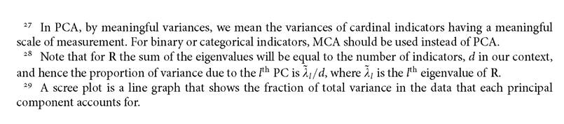

create societal measures. To ease the interpretation of the components, the weights are often rescaled so that those related to the components accounting for a greater proportion of the total variance are larger. The rescaled weights are referred to as component ‘loadings' and may be interpreted as the correlation coefficient(s) between indicator j and component l when the correlation matrix or the standardized covariance matrix is used. In a similar manner, to facilitate the comparison across components, it is often convenient to rescale the components. This is equivalent to standardizing them to have unit variance. This leads to a standardized representation of the l^th PC of person i as

As in section 3.4.2, the dimensional components may be combined into an individual score using a multivariate or an ad hoc procedure, and individual component scores may be aggregated, for example, by using a simple average.

3.4.3.2 Multiple Correspondence Analysis

When the indicators are ordinal, binary, or categorical, a more suitable multivariate technique for a lower-dimensional description of the data is correspondence analysis (CA). The use of correspondence analysis in social sciences increased significantly in the late 1980s, inspired mainly by the work of Bourdieu (1986, 1987). The history of CA can be traced back to the mid-1930s during which various authors defined correspondence analysis in different but mathematically equivalent ways.^[100] An intuitive and widely used definition in the multivariate statistical literature is the geometrical approach suggested in Greenacre (1984) and Greenacre and Blasius (2006) who follow the ideas of the French mathematician and linguist Jean-Paul Benzdcri (Benzdcri and Bellier 1973). This geometric approach sees CA as an adaptation of PCA to categorical data.

Like PCA, CA is based on a geometric decomposition.^[101] Simple correspondence analysis explores the association between two categorical indicators, xj and xj having categories l and l', respectively, using a two-way contingency table or cross-tab of relative

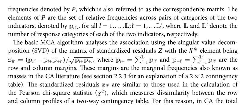
variance in the cross-tab, called ‘total inertia’, is equal to χ² divided by the sample size. Similar to PCA, in CA one also needs estimates of the total inertia (‘variance’) and of the component weights or coefficients to obtain person-specific achievement values. These are obtained from the SVD of Z where the eigenvalues,^[102] called ‘principal inertias’, quantify the variance in the cross-tab and the singular vectors give the axes’ coordinates for the low-dimensional representation and play a similar role as weights or coefficients in PCA. When the reduction in dimensionality involves two axes, one can plot the axes’ coordinates, providing a visual representation (bi-plot) of the association across categories of the indicators.

In the general case of a set of categorical indicators, CA extends the analysis to a multiway table of all associations amongst pairs of variables. This is an MCA, which performs a CA on a Burt or indicator matrix. The indicator matrix I is an individuals-by-categories matrix. The elements of this matrix are 0s and 1s with columns for all categories of all indicators and rows corresponding to individuals. A value of 1 indicates that a category is observed; a 0 indicates that it is not. The Burt matrix is a matrix of all two-way cross-tabulations of the categorical variables. MCA on either the Burt or indicator matrix gives equivalent standard coordinates, but the total principal inertias obtained from each of the two approaches differ.

As with simple correspondence analysis, the principal inertias and the singular vectors are used to obtain person-specific achievement or deprivation values. Thus, the person’s deprivation score will vary depending on whether the Burt or indicator matrix is used. The Burt matrix is the most commonly used.^[103]

3.4.3.3 Factor Analysis and Structural Equation Modelling

Factor Analysis (FA) and structural equation models fit within the broad class of Latent Variable Models (LVM). LVMs are regression models that make assumptions and express relationships between observed and unobserved (or latent) variables. The development of the single-factor model was initiated by Spearman (1904) to measure overall intelligence. This was further generalized by Garnett (1919) and Thurstone (1931), among others. In an FA model, the main assumption is that several observed indicators depend on the same latent variable or variables. This dependence is reflected in the correlation matrix across indicators. Thus FA is a model-based technique that assumes an underlying statistical model regarding the variation in a set of indicators. As discussed earlier, the common variance is represented by a factor. Like PCA, FA is also used as a data reduction method; however, there is a fundamental difference between the two methods. PCA is a descriptive method that attempts to interpret the underlying (latent) structure of a set of indicators on the basis of their total variation, while FA is a model-based method that focuses on explaining the common variance across indicators instead of total variance.

Factor models could be either exploratory or confirmatory. Exploratory factor analysis (EFA) models make no prior assumptions regarding the pattern of relationships among the observed indicators and the latent factors. Confirmatory factor analysis (CFA) models do assume a pre-specified pattern of relationships.

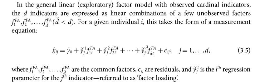
The general linear factor model assumes that the factors have a mean of 0, a variance of 1, and are uncorrelated with each other. It also assumes that the residuals have a mean of 0, are heteroscedastic, and that they are uncorrelated with the factors. The general linear factor model may lead to the normal linear factor model if, additionally, it is assumed that the observed indicators and the residuals follow a multivariate normal distribution.

The essence of factor models is the correlation structure of the model's indicators. This is reflected by the correlation matrix predicted by the model. To fit factor models, one looks for values of the parameters such that the observed correlation matrix is as close as possible to the one predicted by the model. The estimation could be done through a variety of methods comprising generalized least squares and maximum likelihood (cf. Joreskog 1970; Bollen 1989; Joreskog and Sorbom 1999; Muthdn 1984; Muthdn and Muthdn 1998-2012). The adequacy of the model and the selection of the number

of factors to retain are checked through goodness-of-fit statistics (Bartholomew and Tzamourani 1999). When the observed indicators comprise categorical variables it is possible to construct a meaningful correlation matrix. This ‘adjusted' correlation matrix will include standard Pearson correlations for pairs of cardinal indicators, tetrachoric (polychoric) correlations for pairs of binary (categorical) indicators, and bi-serial (polyserial) correlations for pairs of cardinal and dichotomous (categorical) variables. For such purposes, one can assume that a latent continuous variable, normally distributed, underlies every categorical variable. This is referred to as the underlying variable approach (cf. Joreskog and Moustaki 2001).

Following the estimation, and to ease interpretation, the factors are transformed into a ‘new' set of factors. This process is called ‘rotation' and involves orthogonal and oblique rotations, among others. The latter requires relaxing the assumption of absence of correlation among factors.

Once the factors have a meaningful interpretation, it is possible to obtain person-specific achievement values on the latent variable. The prediction of the achievement/deprivation values could be achieved through several methods that lead to highly correlated but different cardinal values of the factor (Bollen 1989). In the presence of only cardinal variables, factor scores often come from regression analysis (see, for example, Lawley and Maxwell 1971). In the presence of binary or categorical variables, factor scores may be computed through Bayesian estimation.

CFA models differ from EFA models as they pre-specify patterns of relationships between the observed indicators and the latent variables. These models extend to structural equation models, which, in addition to the measurement equation, specify relationships across factors and between factors and other explanatory variables. The second type of relationship is referred to as the structural part of the model. Hence in this case the statistical model is composed of two parts: a measurement part and a structural part (Bollen 1989).

Among these models we find the so-called multiple-indicator multiple-causes models (MIMIC), which are characterized by a latent endogenous variable but no measurement error in the explanatory variables. The full structural equation model corresponds to a regression model where both dependent and explanatory variables are measured with error (cf. Bollen 1989; Browne and Arminger 1995; Joreskog and Sorbom 1979). As with EFA, with CFA models one needs to estimate the model, assess its quality of fit, and predict factor scores. Further, one could also be interested in performing statistical inference with the predicted scores. For a discussion of the exact statistical properties of scores resulting from factorial methods, see Krishnakumar and Nagar (2008).

3.4.4 Acriticalevaluation

The strengths of statistical methods that we have presented in this section are several. First, descriptive techniques such as PCA and MCA aim to reduce dimensionality and can be used in an appropriate normative setting to create an aggregate achievement value that can be further used for identification of the poor and for constructing poverty indices. In addition to the reduction of dimensionality, model-based techniques are appropriate when poverty is considered to be an unobserved or latent phenomenon, and the measurement purpose is to specify relationships between the unobserved variables and some observed indicators that are assumed to partially and indirectly measure this abstract concept. Furthermore, statistical techniques are easy to apply, and certain methods can be used with ordinal as well as cardinal data. Also, statistical methods can be used in conjunction with other approaches. For example, PCA, MCA, or FA could be helpful for the selection and categorization of indicators when constructing a multidimensional poverty measure. Thus, statistical methods can complement other methods presented in this chapter.

Despite their strengths, statistical methods have certain limitations when constructing poverty measures. First, it remains unclear which of the axiomatic properties outlined in Chapter 2 these indices do and do not satisfy. As explained in Chapter 2, an understanding of the embedded properties is important in order to follow how a poverty index behaves, given various changes in the joint distribution of achievements or deprivations. As it may not be intuitively easy to understand various properties that indices based on statistical methods may satisfy, further research is required. For example, recall that all statistical methods, in practice, use sample moments. For second-order sample moments, in order to obtain an unbiased estimate of the variance and covariance, we lose one degree of freedom, i.e. instead of dividing by the sample size, we divide by the sample size minus one. This may cause the overall poverty index based on these methods to violate the replication invariance property (section 2.5.1), which would make the comparison of countries with different population sizes very difficult. Measures based on certain statistical applications may violate other axioms such as deprivation focus or monotonicity.

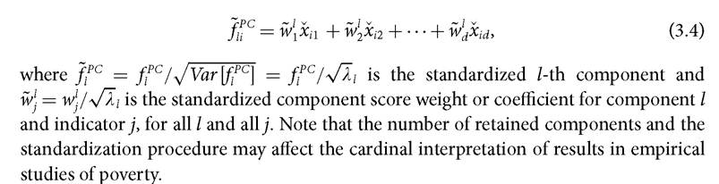
Second, comparisons across different datasets require considerable care when statistical methods are used to create individual achievement values or an overall poverty index. For example, when comparing two countries or time periods using the standardized component score or weights in equation (3.4), one should bear in mind that the comparisons are relative. That is, they depend on the eigen decomposition of the corresponding datasets. Even if datasets are pooled in order to improve comparability, the resulting weights are still relative. For example, suppose that to compare the weights in equation (3.4) across two time periods, one pools two national datasets. Now suppose a third period is added and must be compared with the previous two periods. In order to preserve comparability of weights across all three periods, one now needs to pool all three datasets. But the conclusions for the first two datasets in the three-way pooling may not remain the same as the conclusions when only two datasets were pooled. Hence, the conclusions remain relative even when datasets are pooled.

The assumptions underlying statistical methods also require scrutiny. For example, some descriptive methods capture the associations between dimensions using Pearson's correlation, which is only a linear measure of association and may not always be success­ful in capturing the more complex association structure between dimensions. In the case of model-based methods, one should bear in mind the underlying statistical assumptions, specifically bivariate normality used for computing the tetrachoric correlations. This correlation applies to binary indicators and is used for fitting purposes in the model. But the assumption of bivariate normality may not be an appropriate assumption when indicators are binary (Mardia, Kent, and Bibby 1979).

Another challenge is that it may be difficult to provide an intuitive interpretation of the person-specific achievement/deprivation values or the overall poverty index constructed through PCA or EFA. For example, the well-known person-specific asset index scores that are often used to rank the population may not have an intuitive interpretation, nor may components such as the weights. Thus, in the analysis of poverty using the asset index scores, it is often not possible to set an absolute poverty cutoff to identify the poor. The usual practice is to follow a relative approach, dividing the entire population into percentiles and then identifying the population in the bottom percentiles as ‘poor’.

Finally, as this section has specified perhaps more clearly than in standard expositions of these techniques, the precise applications of statistical methods can vary a great deal, and seemingly minor or incidental methodological choices may affect results. Relevant decisions include the selection of the statistical method, the number of components to retain, the method for combining components (multivariate or ad hoc), the selection of weights to combine factors (e.g. proportion of variance, inverse of variance, or some other approach), and the functional form used to aggregate across individuals. Other choices that may affect results include the selection of the unstandardized or standardized covariance matrix in PCA, the choice of the Burt or indicator matrix in MCA, and the choice of CFA rather than EFA, as well as methods used to rescale weights or generate factor scores, if relevant. The normative basis of such a multidimensional poverty measure could be difficult to ascertain. The reach of statistical approaches could be greatly strengthened if the axiomatic properties were clarified, methodological choices were justified normatively, and the robustness of results to alternative justifiable implementation methods were routinely and transparently assessed.

3.5