The European Union
In a variety of forms the ‘European Union' (EU) has been in existence for almost 50 years. Given the almost continual controversy which has surrounded the issue, it is easy to forget that the UK has been a full member for over 30 years.
This chapter seeks to review the development of the Union and its impact on the UK. It considers all major areas in which the EU now has a role and examines the links between ‘political' goals and economic structures.From European Coal and Steel Community (ECSC 1952-57), to European Economic Community (EEC 1958-86), to European Community (EC 1986-92), to European Union (1993- ) and a single currency (1999), the ‘European idea' has moved inexorably forward, to such an extent that the EU 15 became the EU 25 with the accession of a further 10 countries in 2004 and now 27 with the subsequent accession of Bulgaria and Romania. Each step has taken the idea further from its original ‘pure' economic roots towards more and more explicit declarations of political intent. The fundamental idea behind every step of the European process has been a very simple one: to construct a form of economic and political co-operation which would make future wars between the nations of Europe totally unthinkable. One forgets this ‘fundamental objective' at one's peril.
I Historical background
The historical background to the EU has been covered in some depth elsewhere (see, e.g., Lewis 1993). Since its foundation, the EU has absorbed the two ‘communities’ which preceded it, i.e. the European Coal and Steel Community (ECSC) and the European Atomic Energy Community (Euratom). The ECSC had been established in 1952 to control the pooled coal and iron and steel resources of the six member countries - France, West Germany, Italy, Belgium, the Netherlands and Luxembourg. By promoting free trade in coal and steel between members and by protecting against non-members, the ECSC revitalized the two war-stricken industries.
It was this success which prompted the establishment of the much more ambitious European Economic Community (EEC), subsequently known simply as the European Community (EC). The European Atomic Energy Community (Euratom) had been set up by treaty in 1957 with the same six countries, to promote growth in nuclear industries and the peaceful use of atomic energy.The EEC was formed on 1 January 1958 after the signing of the Treaty of Rome. This sought to establish a ‘common market’, by eliminating all restrictions on the free movement of goods, capital and persons between member countries. By dismantling tariff barriers on industrial trade between members and by imposing a common tariff against nonmembers, the EEC was to become a protected free trade area or ‘customs union’. The formation of a customs union was to be the first step in the creation of an ‘economic union’ with national economic policies harmonized across the member countries. The original ‘Six’ became ‘Nine’ in 1973 with the accession of the UK, the Republic of Ireland and Denmark, and ‘Ten’ in 1981 with the entry of Greece. The accession of Spain and Portugal on 1 January 1986 increased the number of member countries to 12.
With the entry into law of the Single European Act in January 1993 the EC became the European Union (EU). In January 1995 the 12 became 15 as Austria, Finland and Sweden joined, followed by the new EU10 in May 2004 and by Romania and Bulgaria in January 2007, bringing the population of the EU to over 50 million with a GDP of over ˆ12 trillion.
The Single European Act (SEA), as it is widely known, came into force in July 1987. It constituted a major development of the Community and was based on a White Paper, ‘Completing the Common Market’, which had been presented by the Commission to the Milan meeting of the European Council in June 1985. It represented the first time, since 1957, that the original Treaty of Rome had been amended. The Act looked towards creating a single European economy by 1993.
The objective was not simply to create an internal market by removing frontier controls but to remove all barriers to the movement of goods, people and capital. Achieving a single European market has meant, amongst other things, work on standards, procurement, qualifications, banking, capital movements and exchange regulations, tax ‘approximation’, communications standards and transport.Since 1987 over 600 separate new directives have been created, ranging from common hygiene rules for meat and regulations on the wholesaling, labelling and advertising of medicines, to capital adequacy rules for investment and credit institutions and a common licensing system for road haulage. The Single Act also had political ramifications in that it formalized the use of qualified majorities for taking decisions in the Council of Ministers and gave the elected European Parliament greater legislating powers.
The European Economic Area
In the 1990s the political and economic problems of the EU itself prevented formal enlargement but did not stand in the way of intermediate arrangements for closer co-operation with certain states. In 1992 the EU signed an agreement with the seven members of the European Free Trade Association (EFTA) which led, on 1 January 1993, to the formation of the ‘European Economic Area’ (EEA). The EEA then consisted of 19 states which together formed a powerful and wealthy trading bloc.1 Under the agreement, the EU extended to EFTA all of the EU’s own freedoms in the movement of goods, services, people and capital while the EFTA states agreed to abide by the EU’s competition rules. Under agreements existing prior to the EEA agreement, industrial tariffs between the 19 countries were already at zero. The 1992 agreement further reduced agricultural tariffs and established a new EEA fund designed to help the poorer EU regions (including Northern Ireland).
The Maastricht Treaty
The Treaty on European Union which was signed at Maastricht on 7 February 1992 represents one of the most fundamental changes to have occurred in the EU since its foundation.
Although, legally speaking, merely an extension and amendment to the Treaty of Rome, Maastricht represents a major step for the member states. For the first time, many of the political and social imperatives of the Community have been explicitly agreed and delineated. Maastricht takes the EU beyond a ‘merely’ economic institution (if it ever was such) and towards the full political, economic and social union foreseen by many of its founders. Some of its major objectives are as follows:■ to create economic and social progress through an ‘area without internal frontiers’ and through economic and monetary union (EMU);
■ to develop a common foreign, security and defence policy which ‘might lead to common defence’;
■ to introduce a ‘citizenship of the Union’.
Table 27.1 presents some of the important characteristics of the 27 member countries in 2010. It shows how diverse they are in terms of population, industrial structure, standard of living, unemployment level and inflation rate. In terms of population, the UK is still the third-largest member, with a smaller proportion engaged in agriculture than in other EU countries but the fifth largest in services. In overall wealth, however, the UK drops down the rankings. It has the third-largest GDP in absolute terms, but comes only eleventh in terms of GDP per capita.
Quite apart from the political rationale behind the EU, a number of economic arguments have been advanced in its support:
■ By abolishing industrial tariff and non-tariff barriers at national frontiers, the EU has created a single ‘domestic’ market of around 490 million people, with opportunities for substantial economies of scale in production. By surrounding this market with a tariff wall, the Common External Tariff (CET), member countries are the beneficiaries of these scale economies.
■ By regulating agricultural production through the Common Agricultural Policy (CAP), the EU has become self-sufficient in many agricultural products.
■ By amending and co-ordinating labour and capital regulations in the member countries, the EU seeks to create a free market in both, leading to a more ‘efficient’ use of these factors. A further factor, ‘enterprise’, is to be ‘freed’ through increased standardization of national laws on patents and licences.
■ By controlling monopoly and merger activities, competition has been encouraged both within and across frontiers.
■ By creating a substantial ‘domestic’ market and by co-ordinating trade policies, the EU hopes to exert a greater collective influence on world economic affairs than could possibly be achieved by any single nation.
These policies have been supported by a number of other arrangements, including a common form of taxation, a common currency and policies directed towards transport, energy, education, social improvement and regional aid. Although our main concern in this chapter will be economic, we should not overlook the political objectives which lay behind the formation of the EU. As early as 1946, Winston Churchill had called for a ‘United States of Europe’ as a diplomatic and military counter to the Soviet Union. However, it was two Frenchmen - Robert Schuman and Jean Monnet - who were the founding fathers of the EC, with their vision of using economic involvement to tie Europe’s warring countries together. Having attempted, on three occasions, to join the EU during the 1960s, the UK was finally accepted for membership in 1970, signed the Treaty of Accession in 1972, and became a full member with effect from 1 January 1973.
The UK’s objectives in signing the Treaty of Accession in 1972 were a combination of the short- to medium-term economic, with the medium- to longterm political. There was an undeniable desire to share in the prosperity which the EU appeared to have stimulated for its six original members since 1958. The fact that the average growth rate of the Six had been 4.8% per annum between 1961 and 1971, compared to the UK’s 2.7% per annum, seemed to show that entry into the EU might offer a solution to some of the UK’s growth problems.
In this chapter we examine the EU and the effect of UK membership of the EU under five broad headings:Table 27.1 The 27 in 2010: some comparative statistics.
Shares of GDP Shares of EU
---------------------------------- GDP per --------------------------------------------------- Index of
| Member country | Population (m) | Agriculture (%) | Industry (%) | Services (%) | GDP ˆ(bn) | capita 6(000)s | GDP (%) | Population (%) | GDP per capita | Unemployment1 (%) | Inflation (%) |
| Austria | 8.4 | 3 | 29 | 68 | 281.1 | 33.5 | 2.3 | 1.7 | 139.6 | 6.0 | 1.3 |
| Belgium | 10.8 | 1 | 26 | 73 | 345.5 | 32.1 | 2.9 | 2.2 | 133.8 | 9.9 | 1.3 |
| France | 64.8 | 2 | 21 | 77 | 1,992.0 | 30.8 | 16.5 | 12.9 | 128.3 | 10.2 | 1.1 |
| Finland | 5.4 | 3 | 33 | 64 | 180.1 | 30.7 | 1.5 | 1.0 | 127.9 | 10.2 | 1.6 |
| Germany | 81.9 | 1 | 30 | 69 | 2,436.0 | 29.8 | 20.2 | 16.3 | 124.2 | 9.2 | 0.6 |
| Greece | 11.3 | 4 | 20 | 76 | 243.0 | 21.4 | 2.0 | 2.2 | 89.2 | 10.2 | 1.4 |
| Ireland | 4.5 | 2 | 34 | 64 | 160.5 | 35.9 | 1.3 | 0.9 | 149.6 | 14.0 | -0.8 |
| Italy | 60.4 | 2 | 27 | 71 | 1,573.0 | 26.0 | 13.1 | 12.0 | 108.3 | 8.7 | 1.8 |
| Luxembourg | 0.5 | 1 | 16 | 83 | 39.1 | 79.8 | 0.3 | 0.1 | 332.5 | 7.3 | 1.7 |
| The Netherlands | 16.6 | 2 | 25 | 73 | 581.8 | 35.1 | 4.8 | 3.3 | 146.3 | 5.4 | 1.2 |
| Portugal | 10.7 | 3 | 25 | 72 | 164.1 | 15.4 | 1.4 | 2.1 | 64.2 | 10.7 | 1.1 |
| Spain | 46.6 | 3 | 30 | 66 | 1,046.0 | 22.5 | 8.7 | 9.3 | 93.8 | 20.0 | 0.8 |
| EU12 | 321.9 | 2 | 26 | 72 | 9,042.1 | 28.1 | 75.1 | 64.1 | 117.1 | 10.7 | 1.1 |
| Bulgaria | 7.6 | 7 | 31 | 62 | 33.6 | 4.4 | 2.8 | 0.2 | 1.8 | 8.0 | 1.3 |
| Cyprus | 0.8 | 2 | 19 | 79 | 17.8 | 22.1 | 0.1 | 0.2 | 92.1 | 6.6 | 3.3 |
| Czech Rep. | 10.5 | 2 | 39 | 59 | 140.9 | 13.4 | 1.2 | 2.1 | 55.8 | 7.9 | 1.4 |
| Denmark | 5.5 | 1 | 20 | 79 | 230.4 | 41.7 | 1.9 | 1.1 | 173.8 | 15.2 | 1.6 |
| Estonia | 1.3 | 3 | 26 | 71 | 13.4 | 10.1 | 0.1 | 0.3 | 42.1 | 20.0 | 0.8 |
| Hungary | 10.1 | 4 | 30 | 66 | 98.1 | 10.0 | 0.8 | 2.1 | 41.7 | 11.3 | 4.2 |
| Latvia | 2.2 | 3 | 26 | 71 | 16.7 | 7.5 | 0.1 | 0.5 | 31.3 | 19.9 | -3.7 |
| Lithuania | 3.5 | 4 | 33 | 63 | 24.7 | 7.4 | 0.2 | 0.7 | 30.8 | 17.6 | -1.2 |
| Malta | 0.4 | 2 | 19 | bgcolor=white>795.8 | 13.9 | 0.05 | 0.1 | 57.9 | 7.4 | 1.6 | |
| Poland | 38.1 | 4 | 31 | 65 | 327.0 | 8.5 | 2.7 | 7.6 | 35.4 | 9.9 | 2.0 |
| Romania | 21.4 | 7 | 37 | 56 | 122.9 | 5.7 | 1.0 | 4.3 | 23.8 | 8.7 | 3.6 |
| Slovakia | 5.4 | 4 | 39 | 57 | 69.5 | 12.8 | 0.6 | 1.1 | 53.3 | 12.8 | 2.4 |
| Slovenia | 2.0 | 2 | 31 | 65 | 36.3 | 17.9 | 0.3 | 0.4 | 74.6 | 8.3 | 3.9 |
| Sweden | 9.3 | 1 | 28 | 71 | 312.6 | 33.7 | 2.6 | 1.9 | 140.4 | 10.2 | -1.0 |
| UK | 62.2 | 1 | 23 | 76 | 1,858.0 | 29.0 | 12.9 | 12.4 | 104.2 | 8.7 | 1.4 |
| EU27 | 501.9 | 2 | 27 | 71 | 12,048 | 24.0 | 100.0 | 100.0 | 100.0 | 10.3 | 1.2 |
| EU15 | 398.7 | 2 | 26 | 72 | 11,420 | 27.9 | 94.8 | 79.4 | 116.3 | 6.0 | 1.1 |
1Eurostat definition of unemployment.
2Private consumption deflation.
Sources: Adapted from European Commission (2010c) Statistical Annex of European Economy, Spring; World Bank (2010) World Development Indicators, and previous editions; OECD (2010b) OECD Factbook, 2010.
HISTORICAL BACKGROUND 567
1 Finance and the EU budget
2 Policy areas
Competition Agriculture Structural
Trade and balance of payments
Monetary
Commercial and industrial
3 Monetary Union
EMU
Convergence
Single currency (euro)
4 Enlargement
5 Opting out?
For each of these headings we discuss both EU policy in general and how it has affected the UK in particular.
I Finance and the EU budget
Between 1958 and 1970 the EU was financed by contributions from member states which, although politically determined, were still broadly based on the various countries’ ability to pay. However, since 1970 the EU has financed its spending using a system of ‘own resources’, i.e. income it regards as its own as of right. The composition of ‘own resources’ is shown in Table 27.2 and consists of three main sources of revenue. First, Traditional Own Resources (TOR) includes revenue raised from customs duties such as the CET and agricultural duties. Second, ‘VAT’ is revenue from each country up to a maximum of 1% of its domestic VAT tax base. Third, ‘GNP’ is a levy of up to a maximum of 1.24% of the value of GNP in each member country. This levy, which was originally introduced in 1988, is used as a ‘buffer’ to equate EU revenue with its expenditure. In other words, the actual percentage of GNP required can vary according to how much revenue is required to balance the EU budget (e.g. 0.40% of GNP in 1997 but 0.56% in 2010). Finally, the table also includes ‘other revenue’ which consists of revenue from a variety of sources such as interest on late payments, fines, taxes on salaries of employees of EU institutions, etc.
A notable feature of Table 27.2 is the decline in the relative importance of TOR and VAT as sources of revenue and the growth in importance of the GNP element. The impact of trade liberalization on tariff levels (e.g. reductions via GATT rounds) has meant that the total yield from TOR has failed to increase in line with the expansion of world trade, so that the share of TOR in total revenue has decreased. Similarly, the share of VAT in total revenue has also decreased. This is partly because of decisions made by the Commission to decrease the percentage of GNP which acts as the tax base for calculating the VAT paid by member states. For example, the VAT base for member states fell from 55% of their GNP in 1995 to 50% of GNP by 2003 and has now been capped at that level, so the tax base cannot be greater than 50% of GNP. Once the absolute amount of the tax base has been calculated for each country, then a VAT tax rate is applied to this amount in order to arrive at the sum which each member has to pay. The maximum rate of VAT applied to this tax base has also fallen from 1.4% in the mid-1990s to 0.75% in 2003 and to 0.3% by 2010, which has further decreased the revenue derived by the EU from the VAT source. These curbs on the VAT source of
Table 27.2 Sources of revenue for the EU budget (Am and %).
| 2000 | (%) | 2006 | (%) | 2010 | (%) | |
| TOR | 14,564.9 | (16.4) | 14,225.1 | (12.9) | 14,203.1 | (11.7) |
| VAT | 32,554.6 | (36.7) | 15,884.3 | (14.3) | 13,950.9 | (11.5) |
| GNP | 41,593.4 | (46.9) | 80,562.5 | (72.8) | 93,352.7 | (76.8) |
| Total ‘own resources’ | 88,712.9 | (100.0) | 110,671.9 | (100.0) | (100.0) | |
| Other revenue | 674.0 | 1,297.6 | 1,430.3 | |||
| Total revenue | 89,386.9 | 111,969.5 | 122,937.0 |
Source: Adapted from European Commission (2010b) General Budget of the European Union for the Financial Year 2010, January, and previous issues.
Table 27.3 Budgetary expenditure of the European communities (Am).
| Budget heading | 1998 | bgcolor=white>20002002 | 2006 | 2010 | |
| Agriculture | 40,937.0 | 40,993.9 | 45,377 | 50,991.0 | 58,135.6 |
| EAGGF guarantee | 40,937.0 | 36,889.0 | 40,761 | 43,279.7 | 43,701.2 |
| Rural Development (RDP) | - | 4,104.9 | 4,616 | 7,711.3 | 14,431.4 |
| Structural operations | 28,594.7 | 32,678.0 | 32,998 | 35,639.6 | 36,384.9 |
| Structural Funds | 23,084.4 | 28,105.0 | 30,316 | 32,134.1 | 29,521.9 |
| Community Initiatives | 2,558.8 | 1,743.0 | - | - | - |
| Cohesion Fund | 2,648.8 | 2,659.0 | 2,682 | 3,505.5 | 6,854.9 |
| Others | 302.7 | 325.0 | - | - | - |
| Internal policies | 4,678.5 | 6,027.0 | 6,793 | 8,889.2 | 11,342.3 |
| External policies | 4,528.5 | 4,805.1 | 4,895 | 5,369.0 | 7,787.7 |
| Administration | 4,353.4 | 4,703.7 | 5,225 | 6,656.4 | 7,888.5 |
| Other | 437.0 | 4,072.7 | 3,754 | 4,424.3 | 1,398 |
| Total | 83,529.2 | 93,280.4 | 99,042 | 111,969.6 | 122,937.0 |
| Source: As for Table 27.2. |
revenue reflect the view that it is a regressive tax which tends to disadvantage poorer members of the EU because a greater proportion of their national income is devoted to consumption, resulting in a greater tax burden being placed on them than on richer members. As a result of the trends noted above, the importance of the GNP element in EU revenue has increased in order to fill the revenue gap. This is regarded as a more acceptable source because the contributions of the various member countries to the EU budget are more closely related to their affluence, i.e. to their ability to pay as indicated by GNP.
A breakdown of the expenditure side of the EU budget is shown in Table 27.3. During the early years of the new millennium, around 45% of the EU’s total expenditure was spent on the Guarantee section of the European Agricultural Guarantee and Guidance Fund (EAGGF). This Fund is used to subsidize the farming community under the EU’s CAP in various ways. The Guarantee section is responsible for a wide range of price support programmes but has decreased in importance to only 36% of total EU expenditure by 2010.
The second most important expenditure group is ‘Structural Operations’ which accounts for some 30% of EU expenditures in 2010. Most of the Structural Funds are designed to meet the convergence objective by developing effective employment and regional policies in the EU. Other objectives of ‘Structural Operations’ are to improve regional competitiveness and cooperation whilst also providing technical assistance to EU members. Although not shown in Table 27.3, the Structural Fund is made up of four sub-funds:
1 the European Regional Development Fund (ERDF), which aims to reduce the inequality gap between the Community’s regions;
2 the European Social Fund (ESF), which is designed to improve the labour market in member countries by increasing employment opportunities, employment flexibility and equal opportunities for the workforce;
3 the EAGGF Guidance Fund, which helps to adapt the structure of agriculture by encouraging small (less efficient) farmers to leave the land;
4 the Financial Instrument for Fisheries Guidance (FIFG), which helps the restructuring of the fisheries sector.
These Structural Funds are spent on the EU’s three priority-based objectives:
■ Objective 1 covers regions of the EU in which development is seriously lagging behind the EU average. Member countries can apply to the four funds for assistance under this objective.
■ Objective 2 covers regions undergoing economic and social conversion, involving industrial restructuring or urban problems. The ERDF and ESF provide the main funding assistance under this objective.
■ Objective 3 covers whole countries and provides support for the adoption of education, training and employment initiatives. This objective is mostly funded by the ESF.
The remaining part of the Structural Fund, i.e. ‘Community Initiatives’, is designed to stimulate cooperation between EU member states in promoting measures of common interest, e.g. rural development (the expenditures under this heading are no longer recorded separately but are included in the overall Structural Fund).
Finally, the Cohesion Fund is a separate part of the Structural Operations and is designed to help the least prosperous member states of the EU to take part in Economic and Monetary Union. For example, it provides assistance to projects in Greece, Ireland, Portugal, Spain and Poland, such as those which contribute to improvements in the transport infrastructure and transport networks of those countries.
■ ‘Internal policies’ refers to the funds used to help improve EU competitiveness and includes spending on research and development (R&D) projects.
■ ‘External policies’ includes EU foreign aid to states such as the former Eastern bloc countries wishing to progress towards the market economy model.
In 1998 the European Commission reported on the revenue and expenditure aspects of the EU budget (European Commission 1998). On the revenue side it was suggested that the performance of the budget should be assessed on five criteria, namely resources adequacy, equity in gross contributions, financial autonomy, transparency and simplicity, and costeffectiveness. To fulfil these criteria the report proposed changes which would be simpler, fairer and more cost-effective. In particular, there was support for more revenue being derived from members’ GNP contributions. On the expenditure side, the main proposal was to decrease spending on market support policies for agricultural products. Finally, the report suggested that those members with large budget imbalances (i.e. whose contributions are generally greater than their receipts) should be compensated by some form of correction mechanism. For example, Germany, the Netherlands, Austria and Sweden have found themselves with budgetary deficits which are arguably excessive in relation to their relative standards of living within the EU.
The nature of the imbalances problem can be seen from Table 27.4. This table shows the relative shares of member countries in total EU GNP and in relative contributions to the total revenue for the EU budget, together with figures for the imbalances, both in absolute amounts and as a percentage of the country’s GNP (UK figures are net of its rebate). Some important points can be noted from this table. First, the UK had a 13% share of EU GNP but contributed only 8.3% (after rebate) to the total revenue for the EU budget. Second, the UK often had a negative budgetary imbalance with the EU, except in 2001 when it became a net beneficiary because of an unusually high amount of rebate in that year. Third, other countries such as Germany, France, Italy, the Netherlands, Austria and Sweden were also experiencing negative imbalances with the EU. Arguably their situations are less fair in that their negative budgetary imbalance is a much higher percentage of their respective GNPs than for other member states. Germany’s problems have been particularly difficult because, as a wealthy country with a relatively small agricultural sector, it attracts low shares of EU spending on both the Structural Funds and the CAP. Fourth, it is clear that the EU budget continues to generate major financial transfers to Greece, Portugal, Spain, Ireland and Poland - the five countries that receive a substantial amount from the Cohesion Fund. In addition, the Baltic States were also net receivers of income from the EU.
In March 1999, the Berlin European Council reached an agreement on an important communication entitled Agenda 2000: a stronger and wider Europe. This was directed towards stimulating economic growth, increasing living standards and preparing for the enlargement of Europe over the period 2000-06. On the expenditure side of the new financial framework, the Council agreed to ensure that the EU’s budget expenditure would not rise too rapidly (see Table 27.3). On the revenue side, adjustments were to be introduced to ensure that the burden on the least prosperous members would be alleviated by altering the rules on VAT contributions to the EU budget. At the same time, the UK’s rebate would be gradually decreased, and adjustments made to the GNP method of revenue calculation (the base) in order to reduce the contributions of Austria,
Table 27.4 Shares of GDP and EU budgetary balances, 2009.
| Share of EU GDP (%) | Share of EU budget (%) | Net budgetary balance (C million) | Net budgetary balance (% GNI) | |
| Austria | 3.1 | 2.3 | - 431.5 | -0.16 |
| Belgium | 3.8 | 3.4 | -1,452.7 | -0.43 |
| Bulgaria | 0.3 | 0.4 | 642.2 | 1.94 |
| Cyprus | 0.2 | 0.2 | 6.9 | 0.04 |
| Czech Republic | 1.2 | 1.3 | 1,776.8 | 1.38 |
| Denmark | 1.9 | 2.3 | -821.0 | -0.36 |
| Estonia | 0.1 | 0.1 | 582.0 | 4.34 |
| Finland | 1.9 | 1.8 | -430.3 | -0.25 |
| France | 21.3 | 19.9 | -4,739.4 | -0.25 |
| Germany | 26.8 | 18.6 | -8,107.3 | -0.33 |
| Greece | 2.6 | 2.4 | 3,251.5 | 1.41 |
| Hungary | 0.8 | 0.9 | 2,772.1 | 3.16 |
| Ireland | 1.8 | 1.4 | 47.0 | 0.04 |
| Italy | 17.0 | 14.7 | -4,079.3 | -0.27 |
| Latvia | 0.2 | 0.2 | 513.6 | 2.55 |
| Lithuania | 0.2 | 0.3 | 1,510.6 | 5.67 |
| Luxembourg | 0.4 | 0.3 | -82.8 | -0.32 |
| Malta | 0.1 | 0.1 | 11.7 | 0.22 |
| Netherlands | 6.4 | 1.7 | -2,026.2 | -0.36 |
| Poland | 2.6 | 3.0 | 6,488.5 | 2.16 |
| Portugal | 1.9 | 1.6 | 2,248.8 | 1.43 |
| Romania | 1.0 | 1.3 | +1,755.8 | +1.54 |
| Slovakia | 0.7 | 0.7 | 580.2 | 0.93 |
| Slovenia | 0.4 | 0.4 | 261.6 | 0.76 |
| Spain | 11.8 | 10.8 | 1,794.3 | 0.17 |
| Sweden | 2.5 | 1.6 | -704.2 | -0.24 |
| UK | 13.3 | 8.3 | -1,362.9 | -0.09 |
| EU27 | 100.0 | 100.0 | 0.0 | 0.0 |
Note: Imbalances exclude administrative expenditure and include UK correction payments. A positive net balance means that the country is a ‘net beneficiary' from the EU budget while a negative figure means that the member is a ‘net contributor' to the EU budget.
Sources: European Commission (2010a) Allocation of 2010 EU budgets; ECB (2010) Statistics Pocket Book, May.
Germany, the Netherlands and Sweden to the EU budget.
The UK and the EU budget
It must be stressed that the terms ‘net contributor’ and ‘net beneficiary’ relate only to the EU budget and its relatively tiny amounts of expenditure, and not to the members’ total experience within the Community. Merely to say that Germany and the UK have usually been large net contributors to the budget has no bearing upon whether they have or have not benefited overall from membership of the EU. It is also important to understand that being a ‘net contributor’ does not imply a transfer of German or UK funds to the EU. The budget is ‘self-financing’ to the extent that contributions to it are, by treaty, never the property of the member state. It is intended (although the results in practice are very different) to be a reallocation of resources from rich to poor in much the same way as national income tax. However, it is not so much being in the position of a net contributor to the budget that has worried successive UK governments, as the relative size of that contribution.
The calculation of the UK’s net contribution involves the following procedure:
1 customs tariffs paid directly to EU; plus
2 agricultural levies paid directly to EU; minus
3 administrative costs of collecting the above returned to UK government; plus
4 VAT contribution (according to the rate set by Council); plus
5 direct UK government contribution (the GNP element)
equals gross contribution, minus
6 amount due to UK for agricultural support (from Intervention Board); minus
7 Structural Fund payments
equals net contribution (or benefit for some members).
As a major importer of both manufactured goods and food, the UK collects large amounts under items (1) and (2). The VAT rate as a tax on the value added is, of course, fairly closely related to economic activity and therefore the VAT contribution is reasonably proportional across member countries. Summing items (1)-(5) gives the UK’s gross contribution to the EU budget. However, the UK must set against this the revenue it receives for agricultural support programmes, item (6), and for regional and social projects, item (7). Subtracting items (6) and (7) from gross contribution gives the UK’s net contribution (or benefit).
Whereas the UK’s gross contribution is relatively high compared with those of other members, its receipts from the EU budget, items (6) and (7), are relatively low. The UK receives little in terms of agricultural support because the operation of the CAP largely benefits less efficient producers, and not efficient ones like the UK. The modest increase in EU support for regional and social projects in the UK has been insufficient to correct this imbalance. As a result the UK has consistently found itself a net contributor.
The UK’s net contributions to the EU budget are shown in Table 27.5. The fact that the UK was a large net contributor to the EU was addressed as early as 1984 when, under the Fontainebleau agreement of that year, the UK received a ‘rebate’ according to a set formula which the Commission calls ‘a correction mechanism in favour of the UK’. The rebate was reviewed in 1988 and 1992 and on both occasions the European Commission decided that it should be continued. However, as noted above, under Agenda 2000 the UK can expect its net payments to the EU to rise over the coming years, especially in view of the substantial rebates shown in Table 27.5.
Table 27.5 UK net contributions to the EU budget (£m), 1996-2010.
| 1996 | 1998 | 2002 | 2006 | 20103 | |
| Total contribution1 | 6,721 | 8,712 | 6,340 | 8,857 | 9,515 |
| VAT and FRA2 | - 4 | 874 | |||
| UK abatement | -2,412 | -1,378 | -3,099 | -3,569 | -4,218 |
| Total receipts | 4,373 | 4,115 | 3,201 | 4,948 | -4,820 |
| Net contribution | 2,348 | 4,597 | 3,138 | 3,909 | 4,695 |
1Net of VAT, FRA and Abatement.
2Fourth Resource Adjustment.
3Estimates based on 2009/10.
Sources: Adapted from HM Treasury (2009) European Community Finances, May, CM 7640 and previous issues; HM Treasury (2010) Public Expenditure Statistical Analysis.
I Policy areas
1 Competition policy
The theory behind European competition policy is exactly that which created the original EEC almost 50 years ago. Competition brings consumer choice, lower prices and higher quality goods and services. The Commission has a set of directives in this area which are designed to underpin ‘fair and free’ competition. They cover cartels (price fixing, market sharing, etc.), government subsidies (direct or indirect subsidies for inefficient enterprises - state and private), the abuse of dominant market position (differential pricing in different markets, exclusive contracts, predatory pricing, etc.), selective distribution (preventing consumers in one market from buying in another in order to maintain high margins in the first market), and mergers and takeovers. The latter powers were given to the Commission in 1990.
Two of the most active areas of competition policy have involved mergers and acquisitions (see Chapter 5) and state aid. In the former, the power of the Commission was widened in 1998 to increase the range of mergers which can be referred to it.
The amendments of 1998 were further strengthened in May 2004 when new rules under Regulation 139/2004 were passed, including changes in the rules on jurisdiction and strengthening of the Commission’s powers of investigation and enforcement. Although surveys have found that the EU Commission’s decisions have not been politically biased and that economic welfare has been its main criterion (Bergman et al. 2004), EU mergers policy continues to be controversial. For example, in July 2006 the European Court of First Instance (CFI), the competition watchdog, made the unprecedented decision of annulling the EU Commission’s approval of the 2004 merger between Sony Music and BMG. Its judgment was a serious blow to the authority of the EU Commission.
As well as the issue of mergers and acquisitions, the Commission has attempted to restrict the aid paid by member states to their own nationals through Articles 87 and 88 (previously Articles 92 and 93) of the EC Treaty and Articles 4 and 95 of the ECSC Treaty. These Articles cover various aspects of the distorting effect that subsidies can have on competition between member states. However, it is likely that the progressive implementation of Single Market arrangements will result in domestic firms increasing their attempts to obtain state aid from their own governments as a means of helping them meet greater Europe-wide competition. Overall, aid given by member states to their domestic industry has been running at around 2% of their respective GNPs during the 1990s.
In 2009 some ˆ67.4bn was spent by EU members on state aid, equivalent to an average of 0.6% of EU GDP. Most of the subsidies went to manufacturing (59%) and agriculture (23%). Of the new members, Poland tops the list of state subsidies (3.0% of GDP) followed by Malta (2.3%) and Cyprus (2.1%). However, difficulties still arise in that of the ˆ61.6bn spent by EU states on subsidies, 40% is spent by Germany, Italy, France and the UK - arguably giving such economies considerable advantages over ‘cohesion’ countries such as Greece, Portugal, Spain and Ireland, as well as some of the new economies of the EU10.
2 The Common Agricultural Policy (CAP)
When the Treaty of Rome was signed in 1957, over 20% of the working population of the ‘Six’ were engaged in agriculture. In the enlarged EU of 27 countries in 2009 that figure is only 6.1%, ranging from the UK with 1.6% to Poland with 20%. Since one in five of the EU’s workers were involved in agricultural production in 1957, it came as no surprise that the depressed agricultural sector became the focus of the first ‘common’ policy, the CAP, established in 1962. The objectives of this policy were to create a single market for agricultural produce and to protect the agricultural sector from imports, the justification being to ensure dependable supplies of food for the EU and stability of income for those engaged in agriculture.
Both the demand for, and the supply of, agricultural products are, for the most part, inelastic, so that a small shift in either schedule will induce a more than proportionate change in price. Fluctuations in agricultural prices will in turn create fluctuations in agricultural incomes and therefore investment and ultimately output. The CAP seeks to stabilize agricultural prices, and therefore incomes and output in the industry, to the alleged ‘benefit’ of both producers and consumers.
There are, of course, a number of ways of achieving such objectives. Prior to joining the EU, the UK placed great emphasis on supplies of cheap food from the Commonwealth. The UK therefore adopted a system of ‘deficiency payments’ which operated by letting actual prices be set at world levels, but at the same time guaranteeing to farmers minimum ‘prices’ for each product. If the world price fell below the guaranteed minimum, then the ‘deficiency’ would be made up by government subsidy. Under this system the consumer could benefit from the low world prices whilst at the same time farm incomes were maintained. Although the UK system involved some additional features, such as marketing agencies, direct production grants, research agencies, etc., it was by no means as complex as that which has operated in the UK since 1972 under the CAP.
Method of operation
The formal title for the executive body of the CAP is the European Agricultural Guarantee and Guidance Fund (EAGGF), often known by its French translation ‘Fonds Europeen d’Orientation et de Garantie Agricole’ (FEOGA). As its name implies, it has two essential roles: guaranteeing farm incomes and guiding farm production. We shall consider each aspect in turn.
Guarantee system
Different agricultural products are dealt with in slightly different ways, but the basis of the system is the establishment of a ‘target price’ for each product (Fig. 27.1). The target price is not set with reference to world prices, but is based upon the price which producers would need to cover costs, including a profit mark-up, in the highest-cost area of production in the EU. The EU then sets an ‘Intervention’ or ‘guaranteed’ price for the product in that area, about 7-10% below the target price. Should the price be in danger of falling below this level, the Commission intervenes to buy up production to keep the price at or above the ‘guaranteed’ level. The Commission then sets separate target and Intervention prices for that product in each area of the Community, related broadly to production costs in that area. As long as the market price in a given area (there are 11 such areas in the UK) is above the Intervention price, the producer will sell his produce at prevailing market prices. In effect, the Intervention price sets a ‘floor’ below which market price will not be permitted to fall and is therefore the guaranteed minimum price to producers.
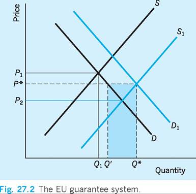
In Fig. 27.2, an increase in supply of agricultural products to S1 would, if no action were taken, lower the market price from P1 to P2, below the ‘Intervention’ or ‘guaranteed’ price, P*. At P* demand is Q' but supply is Q*. To keep the price at P* the EAGGF will buy up the excess Q* - Q'. In terms of Fig. 27.2, the demand curve is artificially increased to D1 by the EAGGF purchase.
If this system of guaranteed minimum prices is to work, then EU farmers must be protected from low- priced imports from overseas. To this end, levies or tariffs are imposed on imports of agricultural products. If in Fig. 27.2 the price of imported food were higher than the EU target price then, of course, there would be no need for an import tariff. If, however,
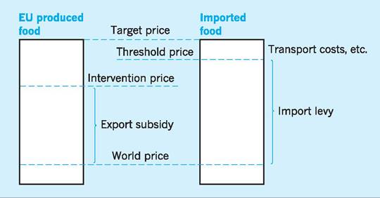
Fig. 27.1 EU agricultural pricing.
the import price is below this, say at the ‘world price’ in Fig. 27.2, then an appropriate tariff must be calculated. This need not quite cover the difference between ‘target’ and ‘world’ price, since the importer still has to pay transport costs within the EU to get the food to market. The tariff must therefore be large enough to raise the import price at the EU frontier to the target price minus transport costs, i.e. ‘threshold price’. This calculation takes place in the highest-cost area of production in the EU, so that the import tariff set will more than protect EU producers in areas with lower target prices (i.e. lower-cost areas).
Should an EU producer wish to export an agricultural product then an export subsidy will be paid to bring his receipts up to the Intervention price (see Fig. 27.2), i.e. the minimum price he would receive in the home market. Problems involving this form of subsidy of oil-seed exports were a major threat to dealings between the EU and the US, with the latter alleging a breach of GATT rules.
Reforms in the latter part of the 1980s had a significant effect on key sectors such as dairy products. In the cereals and oil-seeds market, intervention buying now occurs only outside the harvest periods. Maximum Guaranteed Quantities (MGQs) are also set for most products. If the MGQ is exceeded, then the intervention price is cut by 3% in the following year.
The system outlined above does not apply to all agricultural products in the EU. About a quarter of these products are covered by different direct subsidy systems, e.g. olive oil and tobacco, and some products, such as potatoes, agricultural alcohol and honey, are not covered by EU regulation at all.
Guidance system
The CAP was, as originally established, a simple price-support system. It soon became obvious that agriculture in the ‘Six’ required considerable structural change because too much output was being produced by small, high-cost, farming units. In 1968 the Commission published a report called Agriculture 1980, more usually known as the ‘Mansholt Plan’ after its originator, the Commissioner for Agriculture, Sicco Mansholt. The plan envisaged taking large amounts of marginal land out of production, reducing the agricultural labour force and creating larger economic farming units. The plan eventually led to the establishment of a Common Structural Policy in 1972, which for political reasons was to be voluntary and administered by the individual member states. The import levies of the EAGGF were to provide funds to encourage small farmers to leave the land and to promote large-scale farming units.
Reform of the CAP
The relative failure of the guidance policy has meant the continued existence of many small, high-cost producers in many agricultural areas of the EU, with correspondingly high ‘target’ prices. High target prices have in turn encouraged excess supply in a number of products, requiring substantial purchases by the Guarantee section of the EAGGF, resulting in butter and beef mountains, wine lakes, etc. The net effect of the CAP has therefore been, via high prices, to transfer resources from the EU consumer to the EU producer. At the same time, the CAP has led to a less efficient allocation of resources within the EU in that high prices made the use of marginal land and labourintensive processes economically viable. Arguably, resource allocation has been impaired both within the EU and on a world scale, in that the system of agricultural levies distorts comparative advantages by encouraging high-cost production within the EU to the detriment of low-cost production outside the EU. Finally, through its import levies and export subsidies the CAP introduces an element of discrimination against Third World producers of agricultural products, for whom such exports are a major source of foreign earnings.
The growth of agricultural spending in the early 1980s placed increasing pressure on the EU’s ‘own resources’. By 1983 the 1% VAT ceiling had been breached and even the steady growth in imports (providing CET revenue) was not sufficient to meet the demands on the budget. The member governments were forced to agree to special additional payments to meet deficits which arose in 1983, 1984, 1985 and 1987. With no agreement on reform during the late 1980s, the CAP began to expand rapidly and the Council was forced to agree a series of ‘supplementary’ budgets.
The breakthrough occurred at the Brussels Heads of Government meeting in February 1988 during which a further, new source of finance was sanctioned (up to 1.2% of GNP) in return for legislative limits on the CAP. In 1988 the CAP was limited to a fixed sum of 27.5bn ECU (ˆ27.5bn) and from then onwards could only expand, in future years, by three- quarters of the average rate of growth in EU GNP (see Table 27.6). Other significant limits were placed on the CAP in the form of a ceiling on cereal production (160 million tonnes), a cut in producer prices of about 3% and a new ‘co-responsibility’ levy of 3% on larger farmers.2
The reform of CAP took a further step forward in June 1992 when the so-called ‘McSharry proposals’ for reform were adopted. The purposes of the reforms were, first, to control agricultural production which had been artificially stimulated by CAP; second, to
Table 27.6 CAP spending as a proportion of the EU budget, 1984-2010.
| % of EU budget | |
| 1984 | 65.4 |
| 1988 | 65.0 |
| 1990 | 59.4 |
| 1992 | 53.3 |
| 1996 | 50.4 |
| 1998 | 49.0 |
| 2002 | 41.1 |
| 2004 | 39.0 |
| 2006 | 38.0 |
| 2008 | 35.6 |
| 2010 | 35.5 |
Note: Figures exclude EAGGF guidance.
Sources: As for Table 27.3 and Eurostat (various).
make European agriculture more competitive by reduction of support prices; and third, to discourage very intensive agricultural methods while still maintaining high employment on the land and supporting more marginal and vulnerable farmers.
To achieve these aims, support prices for cereals were to be reduced by some 30%. Also, arable land was taken out of production or ‘set aside’, with farmers receiving payment based on average yields for what is not produced. Livestock farmers were limited to a maximum head of cattle per hectare of available fodder. Other elements of the reform involved direct income-support for farmers in Less Favoured Areas (LFAs) and for those who use environmentally sound methods of farming. Finally, an early ‘pre-pension’ scheme was introduced to accelerate the retirement of farmers who operated unviable holdings.
In July 1997 the European Commission published Agenda 2000 which analysed the EU’s past policies and considered certain long-term future trends. As far as agriculture was concerned, it recognized the need to extend the agricultural reforms of 1992. The recommendations of 1997 were designed to continue the post-1992 trend of reducing price support to farmers (through the intervention buying system) and providing more money payments direct to producers. For example, in the cereals sector the intervention price was reduced by 15% between 2000 and 2002 to set it closer to world levels (see Fig. 27.1). In the milk sector, the intervention price was cut by 15% in three steps from 2005/06 onwards, although output quotas were raised by 1.5% in three steps from 2000 onwards (from 2003 in the UK) to try to alleviate the problems resulting from a lower intervention price.
Finally, a new Rural Development Policy (RDP) was introduced in January 2000 to boost a variety of restructuring schemes directed towards easing these changes in agricultural policy (see Table 27.3). This is the ‘second pillar’ of EU agricultural policy and is designed to help stimulate investment in farm business, develop forestry and forestry products, improve training for young farmers and provide help for those older farmers wishing to retire. In the UK, expenditure on the RDP amounted to £1bn between 2000 and 2006 in support of hard-pressed farmers, given the drop in their incomes resulting from lower intervention prices. In fact, since 2002 the European Commission has been involved in discussions relating to reforming the CAP by freezing agricultural spending from 2007 onwards. It has also introduced the idea of ‘compulsory modulation’ which involves forcing member states to reduce direct payments to agriculture and place more funds into environmental protection and early retirement schemes for workers within the agricultural sector.
Final agreement on the reforms was completed in June 2003 and the implementation by the individual countries took place between 2005 and 2007. The old subsidy system was based on the amount of agricultural output produced, and comprised 11 types of financial support given for growing crops and rearing animals. This system was replaced by a single farm payment (SFP), linked to meeting standards set for the environment, food safety and animal welfare. Recipients will be expected to keep all farmland in good agricultural and environmental condition - this linkage is called ‘cross compliance’. Direct payments to larger farms were designed to be reduced and the money used to help finance the new RDP. Decoupling payments from the output produced means that EU support for agriculture will no longer be classified as ‘trade distorting’, which has been a long-standing criticism of the CAP. However, some member states will retain an element of subsidy in which payments are still linked to output in order to deter farmers from abandoning production and simply taking the single payment for ‘environmentally friendly’ activities.
Payments made to farmers will depend on each farmer’s ‘entitlements’, which are based on how much the farmer received under the old CAP system. However, this type of payment based on ‘historic’ entitlement will be phased out gradually and replaced by the flat rate ‘single payment’ system by 2012. In 2010 UK farmers received around £230 per hectare in SFP payments, as long as they meet standards on the environment, food quality and animal welfare. In the UK, the government expects the new flat rate payment to redistribute subsidies from the more intensive to the less intensive producers, and to land-uses not previously receiving subsidies. Sheep farmers will tend to gain, while beef producers will tend to lose - and in the dairy industry, small producers are expected to gain and large producers to lose. The reformed CAP shows a marked shift of spending towards rural development, where only ˆ7.8m was spent on this area in 2006 as compared to ˆ44.8m on farm subsidies under the CAP. By 2010 the amounts were ˆ14m and ˆ39.2m respectively. In the meantime, the Commission conducted a major review of the CAP in May 2008 to try to make it more efficient. Its proposals included reducing the SFPs to large farms and increasing the funds transferred to the Rural Development budget, and further proposals involved abolishing the set-aside scheme. The CAP is due for renewal in 2013, and it is expected that CAP spending might move towards greater support for innovation, climate and energy. In addition, some proposals have been made to include income insurance schemes for farmers, as 66% of farm earnings are now provided by direct payments from the CAP.
The pressure for agricultural reform has come from many sides - such as consumers who worry that CAP encourages higher prices, ministers afraid of the spiralling budget costs of agricultural subsidies, policymakers aware of the need to shift resources from an EU farming community of 11 million in order to help the 18.5 million Europeans who are unemployed, and supporters of the single currency who accept the need to cut member states’ budget deficits in order to meet the Maastricht criteria. Agricultural reform was also accepted as necessary by supporters of EU enlargement who recognized that if price supports were not decreased, then the enlargement of the EU in 2004 would cause severe budgetary difficulties. This was because farm prices in the new entrants were already 20-40% below the EU level and would require extensive (and costly) support to be raised to the EU levels. Such increases in agricultural prices to EU levels could, of course, also cause financial hardship for the consumers in those lower-income countries, as well as giving a cost-push stimulus to inflation.
3 Structural policy
This is the term given to a combination of what used to be called the Regional and Social Policies (together with several other minor policy areas). For clarity, we have separated these two central policy areas in the discussion which follows.
Regional policy
Like the UK’s own regional policy, the objective of that for the EU as a whole is to attempt to ease regional economic differences (Chapter 23). Almost a quarter of the current EU budget is devoted to ‘regional policy’ as part of what are called the ‘Structural Funds’ (Social plus Regional plus other policies).
Table 27.7 Population covered by EU regional aid, 2007-13.
| Country | Population covered (%) | Country | Population covered (%) |
| Belgium | 25.6 | Denmark | 8.6 |
| Germany | 29.9 | Estonia | 100.0 |
| Greece | 100.0 | Cyprus | 50.0 |
| Spain | 59.6 | Latvia | 100.0 |
| France | 18.4 | Lithuania | 100.0 |
| Ireland | 50.0 | Hungary | 100.0 |
| Italy | 34.1 | Malta | 100.0 |
| Luxembourg | 16.0 | Poland | 100.0 |
| Netherlands | 7.5 | Romania | 100.0 |
| Austria | 22.9 | Slovenia | 100.0 |
| Portugal | 76.7 | Slovakia | 88.9 |
| Finland | 33.0 | Sweden | 15.4 |
| Czech Republic | 88.6 | UK | 21.6 |
| Bulgaria | 100.0 | EU27 | 46.4 |
| Sources: European Commission (2010) Official Journal of the European Union, and various sources. | |||
Regional policy attempts to improve the structural base of the EU’s poorer regions against a background of inequality in income per head, ranging from around 30% of the EU average in some poor regions to over 200% in some rich regions. The disparities in regional income per head have grown still wider with the inclusion of some of the countries in eastern Europe within the EU. Of even greater concern were the findings of an early study by Dunford (1994). This showed that, although the regions of the EU were converging up to 1976, they actually diverged in terms of incomes per head after that date, casting doubt as to the effectiveness of EU regional policy. As a part answer to this problem, a Cohesion Fund was introduced in 1993 to help certain countries achieve the convergence criteria necessary for economic and monetary union. Four countries benefited from the Fund because they had GDP per head of less than 90% of the Community average in the early 1990s. They are Spain (75%), Ireland (68%), Portugal (56%) and Greece (47%). To these are now added Poland. Some ˆ41 bn was spent on this Cohesion Fund over the 1993-2006 time period.
The accepted wisdom during the 1970s and 1980s was that a European core existed which was highly developed and very wealthy. The core consisted of the northern and western parts of Germany, Benelux, most of northern France and south-east England. Outside the core the picture was of a less-developed periphery. It is now understood that the EU’s pattern of economic wellbeing is more patchy and far more complex than the ‘core and periphery’ model.
This core-periphery model has become even more complex with the accession of the EU10 countries in 2004 and the reduced entitlements on offer. For example, the EU had already decided to reduce the proportion of the population eligible to receive regional aid as early as 1997 in order to reduce the value of such subsidies to industry. Over the period 2007-13 the aim is to limit the overall coverage of regional aid to 42% of the population. Table 27.7 provides some idea of the projected coverage of regional aid in the EU27 for the period 2007-13, indicating that the percentage of the population covered by regional aid varies from very low coverage in the Netherlands to very high coverage in the EU10, partly reflecting the lower relative incomes per head shown in Table 27.1. New maps showing the areas covered by regional aid in the various countries have been published since January 2007.
Initially the EU will more carefully scrutinize the eligibility of regions for the Objective 1 status which provides maximum grants, i.e. where GDP per head in the region is less than 75% of the EU average. By 2006, some 50 regions, covering 22% of the EU’s population, had received money under Objective 1, accounting for 74% of the total Structural Fund budget. Meanwhile, 18% of the EU population lived in areas that received Objective 2 money, accounting for 9% of the Structural Fund’s resources. Finally, Objective 3, whose eligibility is not confined to any particular areas of the EU, received 10.3% of total Structural Fund resources.
In the UK, the EU classified Cornwall and the Isles of Scilly, South Yorkshire, West Wales and the Valleys, and Merseyside as areas eligible for Objective 1 funding over the period 2000-06. These areas cover some 5 million people and each has GDP per head levels of around 70% of the EU average. Northern Ireland and the Highlands and Islands received transitional support until 2006 to help them consolidate the improvements they achieved as a result of previous funding in the 1990s.
Social policy
The development of European social policy has involved both the operation of the European Social Fund (ESF) and developments in the ‘Social Chapter’ of the Maastricht Treaty.
The ESF is designed to develop human resources and improve the workings of the labour market throughout the EU. Expenditure is concentrated in those regions of the EU which are suffering from high unemployment and is designed to help with retraining initiatives, improving skills and providing educational opportunities in order to make the labour force more flexible. In March 1998 the European Commission formally adopted a series of draft regulations which formed the backbone of the ESF’s plans for the 2000-06 period. At the centre of these plans was the new European Employment Strategy (EES) which stipulates that each member state must submit an annual employment plan directed towards raising ‘employability, entrepreneurship, labour force adaptability and equal opportunities’. A sum of ˆ210bn was allocated to achieving these goals by 2006.
As far as the ‘Social Chapter’ of the Maastricht Treaty is concerned, the UK had been opposed to many of the regulations and directives associated with the Social Chapter, with successive Conservative governments arguing that attempting to impose regulations in such areas as works councils, maternity/ paternity rights, equal pay, part-time workers issues, etc. merely increased labour costs and decreased UK competitiveness. Nevertheless, the government in the UK has adopted many parts of the Social Chapter in order to provide basic minimum standards across Europe even if this does result in some increase in labour costs. In any case, even if the UK had remained outside the Social Chapter it would still have been subject to a great deal of EU social legislation introduced as part of other programmes from which there is no UK ‘opt-out’. The UK has adopted the Directives such as the Working Time Directive and the Parent Leave Directive in an attempt to catch up with other EU members which had already adopted these directives (see Chapter 14).
4 Trade policy and balance of payments
The EU is the largest trading bloc in the world. It accounts for 19% of world GDP and around 41% of world trade. The EU runs a deficit on its visible trade with the rest of the world, largely due to its need for substantial imports of fuel and raw materials. As regards invisible trade, the EU is roughly in balance with the rest of the world. By the early 1990s, almost 60% of both EU exports and imports involved other EU countries. The growth of this intra-European trade has been a significant factor in attracting inward investment into the EU (see Chapter 7).
The UK's trade with the EU
The UK’s trade with the EU has shown important changes since the late 1960s. First, the area composition of UK visible exports and imports indicates a strong movement towards the Community. In 1969, for example, 29% of total UK visible exports were destined for the EU, whilst 26% of UK visible imports came from the EU. By 2010 the shares had increased significantly, to 57% and 56% respectively. Second, as can be seen from Table 27.8, the UK’s trade with the rest of the EU has shown that the UK had a deficit on trade in goods and services with the EU. Thus there is little real evidence that the UK could earn sufficient income from the EU to cover its large trade deficit, especially in manufactures. Any disadvantage for the UK in its trade in manufactures is particularly worrying, since exports and imports of manufactures together constitute some 66% of total trade with the EU whilst food, drink, tobacco and oil together account for only 25%.
The nature of the EU, as a bloc which allows free trade in manufactured goods, has worked to the
Table 27.8 UK current account transactions with the EU, 1996-2009.
| £m | 1996 | 1998 | 2000 | 2002 | 2005 | 2009 |
| Balances | ||||||
| Trade in goods | - 4,870 | -6,571 | -5,262 | -22,194 | -36,048 | -37,162 |
| Trade in services | -397 | 244 | -1,894 | -1,409 | -1,852 | 9,205 |
| Trade in goods and services | -5,267 | -6,327 | -7,156 | -23,603 | -37,900 | -27,957 |
| Investment income | 1,899 | 7,861 | 6,378 | 18,708 | 11,275 | 19,508 |
| Current transfers | - 6,606 | -6,562 | -5,521 | -4,217 | -5,615 | -5,926 |
| Current account | - 9,974 | -5,028 | -6,299 | -9,112 | -32,240 | -14,375 |
Source: Adapted from ONS (2010c) United Kingdom Balance of Payments, and previous issues.
disadvantage of many relatively less efficient British manufacturers. Similarly, the fact that the EU remains a relatively closed market with respect to both agricultural goods and invisibles (particularly the two areas of relative British strength - insurance and banking) has tended to restrict the UK from taking advantage of the areas in which it has had a small comparative advantage. Table 27.8 shows the UK’s current account transactions with the EU for selected years between 1996 and 2009. The deficit on the goods account continues to be a weakness; whilst trade in services in 2009 has shown significant improvement, it is not clear whether this trend in services will continue. The improvement in the UK’s investment income account has continued with the EU, supporting the idea that it is in her trade balance with the EU that most of the UK’s problems lie as regards current account transactions.
5 Monetary policy
A single currency permitting trade at ‘known prices’ has been a long-standing goal of the EU. Such a currency would overcome the uncertainties created by currency fluctuations which discourage medium- and long-term contracts and therefore international trade. A common currency and common exchange reserves, together with a European Central Bank, are the major features of European EMU. The ‘Snake’, and later the European Monetary System (EMS), were seen by many as steps towards European monetary union.
While now thoroughly integrated into the move towards economic and monetary union, we deal in this section with the background to EMU in the form of the EMS and its precursors and the European Currency Unit (ECU). The discussion of EMU and the euro is presented in a separate section below.
The ‘Snake', 1973-79
Consultations between the ‘Six’ and the three applicant countries between 1970 and 1972 led in 1973 to the establishment of a currency co-operation system called variously the ‘Snake’, or the ‘Snake in the Tunnel’. It required each central bank to maintain its currency within a band of ±2.25% against the US dollar, limiting the fluctuations that could occur between member country currencies. This had the advantage of reducing uncertainty but it did restrict the use of the exchange rate as a policy instrument for adjusting trade deficits and surpluses between members.
The oil crisis of 1973 and ensuing world recession created balance of payments problems for many member countries. Fluctuations in the balance of payments in turn led to more volatile exchange rates, making it more difficult to maintain par values within the narrow bands of the ‘Snake’. As a result, the UK remained a member for only a few months, with France also leaving the system in January 1974. Although the ‘Snake’ itself continued, it did so in a truncated form, with three members outside (UK, the Republic of Ireland and France) and four non-members inside (Norway, Sweden, Austria and Switzerland). In effect, the ‘Snake’ now contained only currencies with a historically close link to the Deutsch mark (DM) and it was replaced in the late 1970s by the EMS.
European Monetary System (EMS) since 1979
The EMS was created in order to increase co-operation on monetary affairs within the Community, and like the ‘Snake’ was founded on the ultimate goal of European Monetary Union (EMU). The EMS was established in March 1979 with three main components, a European currency unit (ECU), an Exchange Rate Mechanism (ERM), and the European Monetary Co-operation Fund (EMCF). In 1989 a fourth element was added - the Very Short Term Financing facility (VSTF). This is a means of funding deficits between member states to an unlimited amount, but for very short periods of time.
The ECU was, possibly, the most radical of the EMS innovations. Whilst superficially similar to the old unit of account in which EU dealings used to be denominated, the ECU was far more than a numeraire. It was valued according to a weighted basket of all the EU currencies. Being a weighted average it was more stable than the exchange rate of any single currency. In addition to its role as a unit of account, it functioned as an international reserve currency. Each member of the EMS ‘bought’ ECUs with 20% of their gold and dollar reserves, which were then held by a new EU institution called the European Monetary Co-operation Fund (FECOM according to its French initials). The central banks used their holdings of ECUs to buy each other’s currencies and to settle debts. Of course, as of 1 January 1999, the ECU was replaced on a one-to-one basis by the euro.
The second element of the EMS involved the ERM which was, essentially, a development of the ‘Snake’. Like its predecessor, the scheme originally set a 2.25% divergence limit, but this time not against the more volatile individual currencies but against the ECU. The new scheme also differed from the old in that it encompassed a formally recognized method of ‘warning’ governments that they have to take action. Each currency had a ‘divergence limit’3 computed against each of the other currencies in the scheme which, because it did not include the ‘home’ currency whose divergence against itself was zero, was always slightly less than the official 2.25% limit. If a currency diverged by more than 75% of this limit it had reached its ‘divergence threshold’ and the government was expected to intervene, either to buy its own currency for ECUs (if the exchange rate has declined) or to sell it for ECUs (if the exchange rate has risen).
The EMCF, the third element in the EMS, consisted of all the heads of the central banks of the member states and was intended to supervise the use of the ‘official ECU’. This was the currency unit originally established, and acted as a means of settling deficits between the members; it was supported by an IMF-type system of deposits of gold and foreign currency. It held the members’ 20% deposits of gold and dollars, was empowered to lend up to 25bn ECUs to countries in difficulties, and was intended ultimately to become a central bank for Europe acting to support the ECU against the dollar, yen, etc.
Until mid-1987 the development of the ECU as a private currency was hampered by the refusal of the West Germans to recognize it. The ECU had been developing as a major international bond currency and, indeed, as a private European currency, but the objections of the West Germans meant that it could not be truly ‘European’. In June 1987, however, the West German government removed their veto on the private holding of ECUs by their citizens and thereby opened the way for further liberalization of capital movements within the Community. Up to 1999 the ECU was used throughout the EU as a basis for travellers’ cheques, and the Belgian government even issued 50 ECU gold and 5 ECU silver coins in 1987 to celebrate the thirtieth anniversary of the founding of the EC. After 1999, the ECU was superseded by the euro.
The UK and the EMS
The UK has always been a member of the EMS but, until late 1990, did not join its exchange rate system (known as the ‘parity grid’). The UK government felt in 1978 that sterling would be too volatile to cope with the confines of the parity grid system. The UK anticipated a continual need to defend a weak pound within the grid, thereby putting pressure on its gold and foreign exchange reserves. The UK also held that the restricted variation in exchange rate against other member currencies would impede the use of the exchange rate as a policy instrument. Finally, by setting limits for sterling, the exchange rate could less readily be used for economic management in the UK, e.g. a high pound helping to curb inflation.
Up to 1987 there had been 11 realignments in the EMS parity grid. The West Germans felt that these readjustments were too frequent, allowing several countries to avoid the macroeconomic discipline originally intended by adopting the system. Ironically, having remained out of the parity grid due to fears of sterling’s weakness, the UK government experienced for a period the exact opposite. At least until the end of 1982 the problem would have been that of having to keep sterling down within the grid rather than of establishing a ‘floor’ for sterling.
There is considerable evidence to suggest that UK trade has become less sensitive to price factors and therefore less easily influenced by exchange rate adjustment. Further, a third of UK trade is still invoiced in the dollar or in other EMS currencies, reducing the importance of EMS currency fluctuations to the UK. For these reasons, it has been suggested that the restrictions imposed on the sterling exchange rate by the EMS parity grid were, from the point of view of trade, less important to the UK than to other EU member countries. It would therefore seem that the restrictions imposed upon UK demand management, via the parity grid, proved the greater deterrent to full UK participation within the EMS. However, the arguments in favour of the UK joining the EMS parity grid became stronger as the EU became more important in UK trade, and as dollarinvoiced oil took a smaller share in UK exports. The problem, once the UK joined in 1990, became the ability of the system to cope with three major currencies, in view of the difficulties it had experienced in coping with two, namely, the DM and French franc.
Black Wednesday
The initial phase of UK membership of the EMS lasted less than two years before the Conservative government of John Major withdrew sterling on Wednesday, 16 September 1992 - ‘Black Wednesday’.
Underlying the events which led to the withdrawal of sterling and the lira from the EMS in September 1992 were two phenomena: the weakness of the US economy and the resulting low interest rates in that country, and the large amounts of capital required by Germany for economic reconstruction in the eastern part of that country and the resulting high interest rates needed in Germany to reduce inflationary pressure. Finance flowed towards the DM and out of US dollars and sterling. The UK government made it worse by refusing to realign sterling in the ERM in early September and there followed two weeks of momentous pressure on European currencies and the ERM itself.
Downward pressure on the Italian lira forced the Italian government first to increase domestic interest rates twice - first to 15% (4 September) and then to 20% (8 September). Continued speculative selling of the lira then forced the Italians to negotiate the first realignment in the EMS since 1987 - a 7% devaluation of the lira against the other EMS currencies (13 September). Finally, a small reduction in German interest rates (by 0.25% on 14 September) was not enough to prevent the lira being withdrawn from the EMS on Black Wednesday.
Sterling followed a similar path to the lira but without the intermediate rises in interest rates. On 3 September the Chancellor announced that the UK was borrowing £7.25bn in foreign currency to assist in the defence of the pound. At the same time, the government made it clear that they had no intention of allowing sterling to be deflected from its rate and band in the EMS. Both German and French central banks, the Bundesbank and the Bank of France, assisted the Bank of England in trying to defend sterling’s central rate in the EMS.
By Wednesday 16 September, however, the financial markets had driven sterling below its ‘floor’ in the EMS and the British government took drastic measures to attempt to maintain sterling’s position. Unprecedented rises in British interest rates - by 2% and then by another 3% (from 10% to 15%) - were announced during Wednesday 16 September, but neither was sufficient to prevent sales of sterling from reducing its rate against the DM well below the EMS ‘floor’ of DM2.78. Sterling was withdrawn from the EMS system - along with the lira - and allowed to ‘float’. Viewed against an EMS central rate of DM2.95 and a ‘floor’ of DM2.78, sterling quickly fell and continued falling. By October 1992 it had reached DM2.36 - a devaluation of some 20% on its previous central rate in the EMS.
These events seemed to indicate that a fixed system of exchange rates could not stand against the sheer scale of currency movements in the new global financial markets. A number of factors might, however, have exacerbated the situation for the EMS in September 1992 which need not have been allowed to hold sway. In the absence of these factors it might have been that the system could have weathered the period in a more effective manner.
It might have been the case that the attempt - unofficially - to ‘fix’ the EMS currencies together as early as the late 1980s and early 1990s was just too early. No realignment had taken place since 1987 in spite of significant underlying economic changes in the economies of the member states (reunification in Germany, lower inflation and better industrial performance in France, high inflation and poor economic performance in Italy, and persistent recession and falling industrial production in the UK). Rather than relieving pressures and differentials gradually by occasional realignments, the EMS had resisted changes in parity for five years. At the same time, unusually large divergencies had built up between the US and German economies. Interest rates of 3% in the US and 9% in Germany carried sufficient differential to create massive currency flows between the two and between Germany and other less successful economies. Large amounts of money were required by the German economy to finance reconstruction, and high interest rates were deemed to be required both to encourage this investment and to keep inflation in check. Political and financial uncertainties over the future of the Maastricht Treaty and, therefore, over the future of EMU following the Danish rejection of the Treaty simply added to the problem.
The crisis in the EMS in September 1992 did not imply that such currency arrangements were impractical or irrelevant, only that the member states of the EU needed to gain more experience of their management. The key seems to lie in achieving the correct balance in the degree of ‘fixity’ of the rates in the system and in ensuring that ‘divergence indicators’ require both strong and weak currencies to take action. Concerns about the degree of ‘fixity’ were met in late 1992 by extending the ERM fluctuation bands to ±15%. This band continued in operation for the non-eurozone currencies after the major EMU reforms of 1999.
6 Commercial and industrial policy
The Common Customs Tariff (CCT) is common to all members of the EU and is imposed on all industrial imports from non-EU countries, though with a few exceptions. Tariff rates differ from one kind of import to another. For example, raw materials and some types of semi-manufactured goods that are not produced within the EU tend to benefit from low duty rates. Tariff rates may also be set at a low rate to stimulate competition within some sectors of the EU, e.g. for pharmaceutical and IT-related goods. Since tariffs on industrial products traded between member countries have been dismantled, the application of the CCT has created a protected free trade area or ‘customs union’ of some 460 million consumers.
The effect of creating a customs union is, however, double-edged. ‘Trade creation’ is the term used to refer to the extra trade between members of the customs union as a result of removing tariff barriers. Production of certain goods is then transferred from high-cost to low-cost producers within the customs union. It can therefore be argued that trade creation causes resources within the customs union to be used more efficiently. However, ‘trade diversion’ also occurs as a result of the CCT imposed against nonmembers of the customs union. This may cause some production to be transferred from low-cost producers outside the union to high-cost producers inside. We shall see below that the two effects are extremely difficult to quantify. However, in general terms, the higher the original tariff between member countries, and the higher the original tariff against nonmembers, the more likely it will be that the efficiency gains from trade creation will outweigh the efficiency losses from trade diversion.
A major study of trade in manufactured goods in France, Germany, Italy and the UK over the period 1985-95 showed a strong ‘trade-creation’ effect from the creation of the Single Market but found little evidence of a ‘trade diversion’ effect (European Commission 1996). For example, while the share of the domestic demand in these countries met from other member states (i.e. intra-EU trade) rose from 16.9% to 21.5% between 1985 and 1995, the share of domestic demand met from outside the EU also increased from 12.7% to 15.6%. In other words, there was a strong trade creation effect (rise in intra- EU trade) and no evidence of a trade diversion effect (fall in extra-EU trade).
UK industry and the EU
It is extremely difficult to evaluate the industrial effects of UK entry into the EU. Certainly the hope on entry was that the UK would secure ‘dynamic gains’ in this sector to offset the expected ‘static costs’ of the net budget contribution and higher food prices. The ‘dynamic gains’ were expected to include a boost to output and productivity from a large, protected market, with its potential for scale economies and greater export opportunities. However, for whatever reason,
Table 27.9 Comparisons of manufacturing output (1970 = 100).
| 1970 | 1975 | 1980 | 1985 | 1992 | 2010* | |
| EU (excluding UK) | 100 | 108 | 133 | 133 | 154 | 179 |
| Germany | 100 | 104 | 122 | 122 | 138 | 174 |
| France | 100 | 108 | 133 | 133 | 157 | 174 |
| Italy | 100 | 107 | 139 | 132 | 160 | 148 |
| UK | 100 | 102 | 110 | 113 | 128 | 137 |
*Second quarter.
Source: Adapted from OECD (2010a) Main Economic Indicators, and previous issues.
there seems little evidence in Table 27.9 of those gains in UK manufacturing output anticipated after entry into the EU in 1973. In fact, the real output of UK manufacturing has grown more slowly than that of the other EU countries.
Lord Kaldor suggested, prior to entry, that the alleged ‘dynamic gains’ might turn out to be ‘dynamic costs’, as the UK market in industrial products became more exposed to its European competitors with the dismantling of tariffs. It may be that the UK joined the wrong type of ‘customs union’! If trade in agriculture and in service activities were freed between member countries, rather than trade in industrial products, then some of the alleged ‘dynamic gains’ might indeed have materialized. In Chapter 1 we noted that the trend towards service activities, though a feature of all advanced economies, has been most marked in the UK. It is arguable that it is in this sector that the UK’s comparative advantages lie. The present industrial policy of the EU, which frees trade in industrial products whilst permitting (along with WTO/GATT) the protection of services, would seem to be to the particular disadvantage of the UK.
I Monetary union
European Economic and Monetary Union (EMU)
As long ago as 1969 the Commission funded the ‘Werner Report’ which acknowledged what it called the ‘political wish to establish economic and monetary union’ and set a target of completion by 1980. Unfortunately the severe economic traumas of the 1970s intervened and it was 1979 before even the first stage - the setting up of the EMS - was accomplished.
In 1988 the Council decided to look into the matter again and set up a Committee under the then EC President, Jacques Delors. That Committee reported in June 1989 and the Council agreed to enter into Stage 1 on 1 July 1990.
The first stage of the Delors Plan - the establishment of a true Single European Market (SEM) - had, of course, already been put in train by the Single European Act of 1987. As the fundamental base of the EMU structure, the Commission felt that it was necessary to set out clearly what the economic benefits would be. They therefore commissioned a group of senior economists, financiers and business people to investigate the issues. The Committee under the chairmanship of Paulo Ceccini reported in 1988.
The Ceccini Report
Although published as a single report, the ‘Ceccini Report’ is simply the summary and conclusions of no fewer than 13 separate economic reports on aspects of the single market. It identifies two types of cost associated with what it calls, in shorthand, ‘nonEurope’, i.e. a Europe of markets separated by physical, technical and fiscal barriers:
■ first, those barriers which have an immediate benefit when they are removed;
■ second, those which will have benefits spread over a period of time.
It should be noted that both types include elements of both static and dynamic benefits.
The parts which made up the ‘Ceccini Report’ examined the single market from the point of view of microeconomic benefits (the removal of non-tariff barriers, economies of scale, X-efficiencies, etc.) and of macroeconomic benefits (the supply-side shock and its effects on GDP, inflation rates, employment, production, etc.).
Using a variety of methods, the Report came up with significant benefits which might accrue to EU members as a result of the Single Market. These included the following:
■ total gains of around 216bn ECU at 1988 prices (between 4.3% and 6.4% of EU GDP);
■ price deflation of an average 6.1%;
■ an improvement to the EU’s external trade of about 1%;
■ an improvement to budget balances of about 2.2%; and
■ around 1.8 million new jobs (a reduction in unemployment of about 1.5%).
The Maastricht agreement set out a planned system for moving towards EMU, including the creation of a system of European central banks to precede the European Central Bank (ECB). The full schedule was delineated in three ‘Stages’.
Stage 1
Theoretically this commenced on 1 January 1993 and involved the creation of an EU ‘Monetary Committee’ whose role included general monitoring and review of monetary matters in EU states and throughout the EU as a whole, providing advice to the Council of Ministers and contributing to the preparation for the European System of Central Banks (ESCB) and the ECB (see below).
Stage 2
In theory, this Stage was to commence on 1 January 1994 with the establishment of a new ‘European Monetary Institute’ to strengthen co-operation between EU central banks, co-ordinate monetary policy, monitor the functioning of the EMS and take over the role of the EMCF. The EMI would seek to obtain a ‘high degree of sustainable convergence’ against four criteria:
1 Price stability. This should be close to the performance of the three best performing members. In a protocol to the treaty ‘close to’ was defined as not more than 1.5% above the average inflation of the three best performers.
2 Government finance. This should adhere to a preordained ‘reference value’ - defined as a government deficit of no more than 3% of GDP at market prices and a government debt of no more than 60% of GDP at market prices.
3 ERM fluctuations. Normal margins of fluctuation should not have been breached for two years.
4 Durability of convergence. This was to be measured by long-term interest rate levels. The rate for long-term government bonds should not have exceeded by more than 2% those of the three best performing countries.
The Maastricht Treaty required that the EMI should specify - by 31 December 1996 at the latest - the regulatory, organizational and logistical framework for the ESCB (to be created in the third stage). It should also set a date for the beginning of the Third Stage. If this date was not set before the end of 1997 it would, according to the Treaty, automatically begin on 1 January 1999.
Stage 3
This stage included the establishment of the ESCB which would hold and manage the official reserves of all the member states. At this stage, exchange rates would be fixed and the ECU would acquire full status as a currency throughout the Community. The ESCB would prepare for the establishment of the ECB which, when founded, would have the exclusive right to issue banknotes throughout the EU. It would accomplish this through the central bank of each of the member states. It would receive some 5bn ECU together with all members’ reserves - excepting only member states’ foreign currency, ECU holdings, IMF reserve positions and special drawing rights (SDRs). Any reserves over 50bn ECU in value would also be left with the member country (in theory, of course, these would not be required and could be used in any way by the member state). The theoretical total reserves to be held by the ESCB would, therefore, be around 600bn ECU.
Maastricht established the shape and format of all of the institutions it envisaged. The Treaty provided for it to come into force on 1 January 1993 or on the date on which the last member country deposited an instrument of ratification with the Commission.
There were a number of protocols to the Maastricht Treaty involving most of the members. The UK had a lengthy protocol agreed which allowed it not to proceed to Stage 3 if it did not wish to and excluded it from most of the Stage 2 arrangements (in return the UK would not be allowed to have a vote in Council on arrangements to do with the ESCB or the ECB).
The path to EMU settled down into the following timetable:
1996-98 All member countries brought their economies into line to meet the Maastricht criteria (see Table 27.10).
1998The countries which formed the first members of EMU were selected.
1999January 1 - the EMU process began with the launch of the euro and the beginning of the transition phase (through to the end of 2001). During this phase national currencies still existed but were irrevocably fixed to each other and to the euro.
2002 January 1 - the euro was introduced in coin and note form. A period of six months was allowed for national currencies to be withdrawn from circulation. Since 1 July 2002 only the euro has been legal tender in EMU member countries.
Single currency: the euro
The launch of the single currency, the ‘euro’, occurred on 1 January 1999, although it did not become a physical currency until 1 January 2002 (see also Chapter 20). However, from 1999 onwards the euro became a legal currency in its own right and the vehicle for electronic and business-to-business transactions throughout the eurozone. As early as January 1999 some 25% of Barclays Bank customers had already been asked to invoice or pay in euros.
The long-term effects of the euro, and with it EMU, are to change the nature of the way business is carried out in Europe. For consumers, prices are more ‘transparent’, making it easier to see whether different prices are being charged for the same product in various EU countries. For manufacturers and other traders, the introduction of EMU means the elimination of exchange rate risks, which should benefit smaller businesses which often lack the resources for foreign exchange management.
The EMU might also produce further corporate rationalization as firms merge in an attempt to grow larger in order to derive scale economies from operating within the Single Market. The foreign exchange market is restricted in its dealings as fewer currencies are traded, with most dealings being in currencies outside the euro, together with euro-dollar or euroyen. It is likely that a new market for government debt denominated in euros and a new pool of eurodenominated equity will be created.
For the potential benefits of the euro and EMU to be realized in the long run, three factors will be decisive:
1 Sustainable economic convergence. For the smooth working of the euro, the economies of the participating countries must be in the same stage of the economic cycle and be relatively homogeneous.
2 Strong political commitments to EMU discipline. The European Council of Economic and Financial Ministers (ECOFIN), consisting of the finance ministers of the EU, is able to impose severe fines on member states whose budget deficits exceed the ratio of 3% of GDP. The fines could, as noted above, reach as much as 0.5% of GDP.
3 Credible European Central Bank (ECB). The ECB’s independence is enshrined in the Maastricht treaty, as is its commitment to price stability. Short-term interest rates are set with a view to achieving such price stability. However, political pressure for reflationary policies might arise if the EU experiences slow growth and high unemployment.
The question also remains as to how the national central banks will operate under EMU. Together with the ECB, the national central banks formed the ESCB in June 1998. This body, through its Governing Council and Executive Board, defines and implements monetary policy and foreign exchange and reserves policies. However, the operational responsibility to carry out agreed ESCB policy is retained by the national central banks. As with the federal central banking systems of the US and Germany, the operations of the ESCB are therefore highly decentralized. There is a risk that the national central banks may try to pressurize the independent ECB to adopt policies directed towards growth and employment in situations where the ECB might be more inclined to tighten control of inflation.
Convergence and the Growth and Stability Pact (GSP)
In March 1998 the European Commission announced that 11 members had reached a sufficient degree of sustainable convergence as measured against the Maastricht Treaty criteria. The relevant criteria were (1) consumer price inflation must not exceed that of the three best-performing countries by more than 11 percentage points; (2) interest rates on long-term government securities must not be more than 2 percentage points higher than those in the same three member states; (3) the financial position must be sustainable. In particular, the general government deficit should be at or below the reference value of 3% of GDP, or, if not, it should have declined substantially and continuously and reached a level close to the reference value, or the excess over the reference value should be temporary and exceptional. The gross debt of general government should be at or below 60% of GDP or, if not, the debt ratio should be sufficiently diminishing and approaching the 60% reference value at a satisfactory pace. The exchange rate criterion is that the currency must have been held within the normal fluctuation margins of the ERM for two years without a realignment at the initiative of the member state in question. Based on these figures it was agreed that 11 members of the EU had reached a sufficient degree of sustainable convergence against the criteria laid down in the Maastricht Treaty. The countries which qualified and wished to join the single currency in January 1999 were Austria, Belgium, Finland, France, Germany, Ireland, Italy, Luxembourg, the Netherlands, Portugal and Spain. Sweden and Greece did not meet the convergence criteria at that time and the UK and Denmark had already decided not to take part in Stage 3 of EMU in 1999.
The European Commission’s convergence report of March 2000 concluded that Greece had met the criteria for entering the EMU and Greece was subsequently accepted as a full member from January 2001. Sweden was deemed not to have met the criteria on convergence since its legislation was not compatible with the Treaty and the ESCB Statute, and also its exchange rate had been outside the ERM II and hence fluctuated against the ERM currencies. The UK and Denmark had decided not to take part in Stage 3 of EMU in 1999 and thus remained outside ‘Euroland’.
To maintain stability in Euroland, a ‘Growth and Stability Pact’ has been operating since January 1999 which is designed to ensure that the euro maintains its value over time by committing the participating countries to form ‘convergence contracts’. These contracts are necessary to make sure that members of Euroland continue to maintain their economies under the same economic criteria as when they entered. In particular, the Pact was designed to ensure that the medium-term budgetary discipline criteria were met. At least every two years, the Commission and the ECB report to the Council on the fulfilment of the convergence criteria. If member states exceed the criteria for government budget deficit (set at 3% of GDP) or government debt (set at 60% of GDP) they would be penalized. Penalties for excessive government deficits can involve members having to lodge with the Commission a fixed, non-interest bearing deposit of 0.2% of the country’s GDP and a variable non-interest bearing deposit of 0.1% of GDP for every 0.1% excess over the deficit criteria, up to a ceiling of 0.5% of GDP. The penalty for excessive government debt is a fixed amount involving a noninterest bearing deposit of 2% of a country’s GDP.
The rationale for introducing budgetary discipline in the form of ‘fiscal rules’ as the major part of the GSP included the following.
1 There was a need to correct the so-called ‘deficit bias’ of fiscal policy, i.e. bureaucrats are inclined to spend more than they can afford in the present, and pass the burden of this spending onto future taxpayers. For example, in the mid-1990s, fiscal deficits of 4-5% of GDP were common and these continuously large deficits led to debt as a percentage of GDP rising from 35% in 1980 to 75% by the mid-1990s. To finance such large deficits means that interest rates need to be increased, which in turn cuts back investment and growth.
2 High deficits and debts also have an effect on monetary policy, because fiscal expansion boosts domestic demand and may give rise to inflationary pressures which may require higher interest rates and reduced money supply to curb them.
3 Fiscal rules may also be needed to help stabilize an individual economy because monetary policy is undertaken by the ECB for all countries in the eurozone. In other words, individual countries only have their own fiscal policy to deal with their particular problems and fiscal rules may be necessary to make sure that countries do not expand their budget deficits too much in their attempt to correct an economic downturn.
The actual performance of EU countries, vis-a-vis the GSP ‘rules’, has changed over time. For example, in 1993, when the Maastricht treaty entered into force, the deficit ratio of the euro area stood at a peak of 5.5% of GDP and this was reduced to 3% in 1997,
the year identified for meeting the Maastricht convergence criteria. Fiscal balances improved considerably between 1997 and 2000, but when growth slowed down after 2000 the fiscal balances of some countries quickly deteriorated. Portugal was first to breach the 3% reference value in 2001, and Germany and France followed in 2002, the Netherlands and Greece in 2003, and Italy in 2004. Table 27.10 shows the position for all the 27 countries in 2009 following the
Table 27.10 Performance of the member states in relation to the convergence criteria, 2009.
| Inflation HICP (%) 2009 | Deficit (% of GDP)* 2009 | Debt (% of GDP) 2009 | ERM member 2005 | Long-term interest rate 2009 | |
| Reference value | 1% | 3% | 60% | ||
| Belgium | 0.0 | -6.0 | 96.7 | yes | 3.0 |
| Germany | 0.2 | -3.3 | 73.2 | yes | 2.4 |
| Greece | 1.3 | -13.6 | 115.1 | yes | 10.7 |
| Spain | - 0.2 | -11.2 | 53.2 | yes | 4.0 |
| France | 0.1 | -7.5 | 77.6 | yes | 2.7 |
| Ireland | -1.7 | -14.3 | 64.0 | yes | 5.3 |
| Italy | 0.8 | -5.3 | 115.8 | yes | 3.8 |
| Luxembourg | 0.0 | -0.7 | 14.5 | yes | 2.7 |
| Netherlands | 1.0 | -5.3 | 60.9 | yes | 2.6 |
| Austria | 0.4 | -3.4 | 66.5 | yes | 2.8 |
| Portugal | - 0.9 | -9.4 | 76.8 | yes | 5.3 |
| Finland | 1.6 | -2.2 | 44.0 | yes | 2.6 |
| Czech Republic | 0.6 | -5.9 | 35.4 | no | 3.6 |
| Denmark | 1.1 | -2.7 | 41.6 | no | 2.5 |
| Estonia | 0.2 | -1.7 | 7.2 | no | 3.9 |
| Cyprus | 3.3 | -6.1 | 56.2 | no | 4.6 |
| Latvia | 4.2 | -9.0 | 36.1 | no | 10.0 |
| Lithuania | 4.0 | -8.9 | 29.3 | no | 5.2 |
| Hungary | 1.8 | -4.0 | 78.3 | no | 7.1 |
| Malta | 4.0 | -3.8 | 69.1 | no | 4.0 |
| Poland | 0.9 | -7.1 | 51.0 | no | 5.6 |
| Romania | 5.6 | -8.3 | 23.7 | no | 7.2 |
| Bulgaria | 2.5 | -3.9 | 14.8 | no | 6.0 |
| Slovenia | 0.9 | -5.5 | 35.9 | no | 3.7 |
| Slovakia | 0.9 | -6.8 | 35.7 | no | 3.7 |
| Sweden | 1.9 | -0.5 | 42.3 | no | 2.7 |
| UK | 2.2 | -11.5 | 68.1 | no | 2.7 |
| EU27 | 1.0 | - 6.8 | 73.6 | — | 4.3 |
*A negative sign for the government deficit indicates a surplus.
Sources: Eurostat (2010) Euro indicators; ECB (2010) Statistics Pocket Book, May.
financial shock in 2007/8. Almost all the countries were in breach of the 3% reference, with the average for the 27 countries being 6.8% and the UK’s deficit nearing twice the average. With regards to the debt- to-GDP ratio, some 12 countries were breaching the 60% reference value in 2009, with Italy, Greece, Belgium, France and Germany, amongst others, showing figures of over 70%.
Problems with the Growth and Stability Pact (GSP)
Three main problems have been identified for the GSP.
1 Excessive rigidity. For example, the 3% deficit limit on each country does not take into consideration important variables such as the stock of public debt, the need for infrastructure investment, or the population age structure - all of which affect the demand for fiscal spending. Hence, the operation of a single figure of 3% as the maximum budget deficit for all economies is too rigid. Another rigidity arises because the GSP focuses on annual budgets and therefore overlooks longer- term relationships. For example, governments may be forced to postpone structural reforms, e.g. a pension system that would yield benefits only in the medium-to-long term, in order to meet the annual ‘fiscal rule’.
2 Limiting discretionary fiscal policy which governments may wish to introduce to help their economy. Germany had to struggle to reduce expenditure and to raise taxes whilst on the brink of a recession in 2003.
3 Lacking credibility. The sanctions are decided by ECOFIN, i.e. the economic and finance ministers of the eurozone, in which political motivation has high priority as seen when France and Germany broke the rules in 2003 where no fine was imposed.
The new Growth and Stability Pact
Various problems with the GSP led to its reform in March 2005 in an attempt to meet some of the criticisms outlined above (ECB 2005). The new SGP introduced differentiated ‘medium term objectives’ (MTOs), which take into account the economic characteristics of each country, especially in relation to the debt-to-GDP ratio. These MTOs will be measured in cyclically adjusted terms, i.e. net of one-off and temporary measures to make sure that the focus is on the underlying structural budget position and not on the simple annual budgetary situation as in the original SGP. Second, under the SGP a deficit above 3% of GDP will not necessarily be considered excessive if it can be shown that the breach is ‘exceptionally temporary’, e.g. a deficit can be considered exceptional if it results from a ‘severe economic downturn’. The new GSP provides a list of factors which will be taken into account if the deficit is above 3%, unlike the original GSP. However, the new provisions might make it more difficult to harmonize monetary and fiscal policy and therefore force the ECB to strengthen its stance on interest rates (Al Eyd and Gottschalk 2005).
As a result of the global crisis in 2008, the European Commission adopted an ambitious reform of the pact in July 2010, designed to prevent fiscal ill-discipline. All eurozone members must specify medium-term budget objectives and the growth of public spending must be kept below the medium-term growth of GDP until the target is met. Countries are also required to implement ‘best practice’ budgetary procedures, such as medium-term planning, fiscal rules, etc. In addition, there is an explicit budget deficit limit of 3% of GDP and a target public debt ratio of 60% of GDP. All countries that exceed the debt limit are required to reduce their debt every year at a rate of one-twentieth of the excess debt. For example, a country with a debt of 100%, and thus some 40% from the target, will need to cut the debt by two points (40/20) of GDP every year.
Violation of either budget deficit or debt requirements leads to an ‘infringement process’ and a fine of 2% of GDP if countries do not comply. In addition, the Commission also envisaged monitoring countries using ‘vulnerability indicators’ such as private and public debt, competitiveness, productivity growth, the current account and credit expansion. The Commission will open another infringement procedure for ‘excessive imbalances’ if the country fails to introduce corrective measures - possibly resulting in a fine of 0.1% of GDP.
Advantages/disadvantages of a single currency
A number of advantages have been claimed for the single currency.
■ Lower costs of exchange. Importers no longer have to obtain foreign currency to pay exporters from the eurozone.
■ Reduced exchange rate uncertainty. All members face fixed exchange rates within the eurozone.
■ Eliminates competitive depreciations/devaluations. Historically, countries have tried to match any fall in the exchange rates of rival countries, with such ‘competitive depreciations’ creating uncertainty and discouraging trade.
■ Prevents speculative attacks. Speculators can sometimes force individual currencies to depre- ciate/devalue their currency by selling large amounts of that currency. The euro, being supported by all member countries, is much better equipped to resist such speculative attacks.
However, critics of the euro point to a number of disadvantages:
■ Loss of independent exchange rate policy. Governments can no longer seek to remedy a balance of payment deficit with a member of the eurozone by lowering their exchange rate, thereby making exports cheaper in that country and imports dearer from that country.
■ Loss of independent monetary policy. The eurozone has a ECB which determines the money supply and interest rate policy for all member countries.
Conclusion
The purely economic effects of British membership of the EU are extremely difficult to isolate and describe. It is increasingly irrelevant to speak of economic models of what the UK’s experience might have been if we had not joined the EEC in 1973.
The economic debate has centred around two different ‘models’:
1 the UK as a permanent and irrevocable member of the EU; and
2 the UK outside the EU - the ‘non-Europe’ model.
The viability of any economic argument which describes the UK outside the EU has become more and more suspect as the financial, economic and business environments have become intermeshed since the 1980s. There is little doubt that the UK has experienced a continuing budget deficit with respect to the EU, that its consumers may have suffered a slight welfare loss with respect to food and the policies of the CAP, and that there has been an observable displacement of UK-manufactured goods in our own domestic market.
Alongside these factors one must recognize the interdependence of the member states in almost every commercial and economic area. The EU represents the UK’s most important trading partner by far in both visible and invisible trade. Membership of the Community has also been responsible for significant amounts of inward investment from Japan and the US into the UK. Ironically this inward investment has been so large that the UK is becoming a major exporter of motor vehicles and electronic equipment, developing trade surpluses with the EU in these categories. In a similar fashion, London’s place as one of the pre-eminent financial centres in the world rests strongly on its position as the financial centre in which US, EU and Japanese banks and investment houses come together. Where portfolio investment is concerned, the EU has become much more important to the UK (see Chapter 7).
The UK’s experience in the EMS has been fraught with problems, but it is clear that a number of those problems were of the UK’s own devising. International freedom in financial markets meant that - even outside the EMS - the UK had to ensure that sterling ‘shadowed’ the DM.
However, a further question has to ask why the benefits to the UK have been less than those which have accrued to other members. The UK has not gained massive benefits from Social and Regional Funds and has a relatively efficient agricultural sector. There have been few or no net real benefits from the CAP and we have suffered from having a relatively inefficient manufacturing sector which has been only modestly successful in exporting to Europe. The UK has not, therefore, gained proportional benefits from the free trade area. Outside the EU, however, the UK would still have had to survive, had to manage its own agriculture and had to find markets for its exports in a world in which the ties of the Commonwealth and EFTA would almost certainly have counted for less and less as the years went by.
Key points
■ In 2010 there were 27 member states within the EU. The 27-member EU is essentially a regional trading bloc with 501 million people within a protected free trade area, with a high per capita income of ˆ27,900 per annum.
■ The EU is the largest trading bloc in the world. It accounts for 19% of world GDP and around 41% of world trade.
■ Since 1992, the EU has established the European Economic Area (EEA) which initially included 19 countries altogether.
■ Agriculture is the most regulated sector within the EU. Around 42% of the entire EU budget is spent on various price support and intervention policies involving agricultural products.
■ The Regional and Social Funds are targeted at poorer regions within each member state in order to relieve unemployment and poverty.
■ The Social Chapter includes a number of ‘directives’ establishing minimum working conditions, though the UK has an ‘opt-out’.
■ The Maastricht Treaty in 1992 sought to widen the scope of the EU beyond a common market (see Chapter 26) to that of an economic and monetary union (EMU).
■ Various ‘convergence criteria’ needed to be fulfilled before countries could join EMU, which began on 1 January 1999. These convergence criteria included consumer price inflation within 1∣%, and long-term interest rates within 2% of the average achieved by the ‘best three’ EU countries. In addition, the public sector borrowing requirement (PSBR) should be no higher than 3% of GDP and total public debt no more than 60% of GDP.
■ The Growth and Stability Pact (GSP) aims to maintain fiscal prudence in the EU. A new framework was introduced in 2005 to control excessive budgetary deficits. However, this has been revised in 2010 following the ‘strains’ experienced in operating the GSP during the major financial problems from 2008 onwards.
Now try the self-check questions for this chapter on the Companion Website. You will also find useful links to relevant websites.
Notes
1 The European Economic Area comprised the (then) 12 members of the EU plus Iceland, Norway, Sweden, Finland, Switzerland, Austria and Liechtenstein, though in 1995 Sweden, Austria and Finland joined the EU.
2 The ‘co-responsibility’ levy is a method by which farmers are penalized for over-production of agricultural products. Up to a certain level of production the farmer is entitled to sell his goods either on the open market, or to the EU’s Intervention stocks. Above that, agreed, level of production the price allowed to the farmer reduced by a specific percentage called the ‘co-responsibility’ levy.
3 The divergence limit for any currency was calculated by the formula ±2.25 (1 - w) where w was the percentage weight of the currency in the ECU. For Germany this resulted in a limit of 2.25 (1 - 0.301) = 1.57%.
References and further reading
Ackrill, R. (1997) Economic and Monetary Union, Developments in Economics, Vol. 13, Ormskirk, Causeway Press.
Al Eyd, A. and Gottschalk, S. (2005) The Stability and Growth Pact and slow growth in Europe, National Institute Economic Review, April 192(2): 23-32.
Barnes, I. and Barnes, P. (1995) The Enlarged European Union (2nd edn), London, Longman. Barras, R. and Madhavan, S. (1996) European Economic Integration and Sustainable Development, London, McGraw-Hill.
Benassy-Quere, A. and Coeure, B. (2010) Economic Policy, New York, Oxford
University Press.
Bergman, M. A., Jakobsson, M. and Razo, C. (2004) An Econometric Analysis of the European Commission’s Merger Discussions, Department of Economics, Working Paper Series No. 6/2003, Uppsala University.
Brittan, L. (1994) Europe - The Europe We Need, London, Hamish Hamilton.
De Grauwe, P. (2000) The Economics of Monetary Integration (4th edn), Oxford, Oxford University Press.
Dunford, M. (1994) Winners and losers: the new map of economic inequality in the European Union, European Urban and Regional Studies, 1(2): 95-114.
ECB (2005) The reform of the Stability and Growth Pact, ECB Monthly Bulletin, August, 57-74.
ECB (2010) Statistics Pocket Book, May, Frankfurt, European Central Bank.
European Commission (1996) Economic evaluation of the internal market, European Economy, 63(4): 1-173.
European Commission (1997) Trade patterns inside the single market, The Single Market Review, Subseries IV, Vol. 2, Kogan Page/ Earthscan.
European Commission (1998) Financing the European Union, 7 October, Brussels, Commission of the European Communities.
European Commission (2010a) Allocation of the 2010 EU Budgets, January, Brussels, Commission of the European Communities.
European Commission (2010b) General Budget of the European Union for the Financial Year 2010, January, Brussels, Commission of the European Communities.
European Commission (2010c) Statistical Annex of European Economy, Spring, Brussels, Commission of the European Communities. Eurostat (2010) Economic Indicators, Brussels, European Commission.
Geradin, D., Layne-Farrar, A. and Petit, N. (2011) EU Competition Law and Economics, Oxford, Oxford University Press.
Giavazzi, F. and Blanchard, O. (2010) Macroeconomics: A European Perspective, Financial Times/Prentice Hall.
Goodman, S. F. (1996) The European Union (3rd edn), London, Macmillan.
Griffiths, A. (1992) European Community Survey, London, Longman.
HM Treasury (2009) European Community Finances, May, CM 7640, London.
HM Treasury (2010) Public Expenditure Statistical Analysis, London.
Johnson, C. (1996) In with the Euro, out with the Pound, London, Penguin.
Kenen, P. (1995) Economic and Monetary Union in Europe, Cambridge, Cambridge University Press.
Krugman, P. and Obstfeld, M. (2010), International Economics: Theory and Policy, Financial Times/Prentice Hall.
Leveque, F. and Shelanski, H. (2009) Antitrust and Regulation in the EU and US: Legal and Economic Perspectives, Cheltenham, Edward Elgar. Lewis, D. W. P. (1993) The Road to Europe: History, Institutions and Prospects of European Integration 1945-1993, New York, Peter Lang. McDonald, F. and Dearden, S. (eds) (1998) European Economic Integration (3rd edn), Harlow, Addison Wesley Longman.
Mercier, P. and Papadia, F. (2011) The Concrete Euro: Implementing Monetary Policy in the Euro Area, Oxford, Oxford University Press.
OECD (2010a) Main Economic Indicators, Paris, Organisation for Economic Cooperation and Development.
OECD (2010b) OECD Factbook 2010, Paris, Organisation for Economic Cooperation and Development.
ONS (2010c) United Kingdom Balance of Payments - The Pink Book, London, Office for National Statistics.
Rosamond, B. (2000) Theories of European Integration, London, Palgrave Macmillan. Wistrich, E. (1994) The United States of Europe, London, Routledge.
Wolf, M. (1996) Thinking the unthinkable, Financial Times, 18 June.
World Bank (2010) World Development Indicators, Washington DC.
The following websites are relevant to this chapter:
DTI’s website for Europe and world trade http://webarchive.nationalarchives.gov.uk/+/ http://www.dti.gov.uk/ewt/intro.htm