Soundness Examples

In Chapter 2 we looked at a handful of justification logics: LP and various sublogics in Section 2.6, and other less common justification logics in Sec­tion 2.7. We now examine Fitting models for these justification logics, and verify soundness.

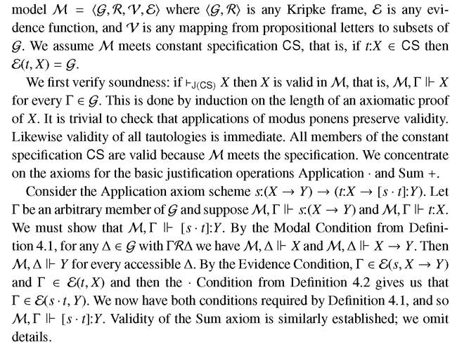
4.3.1 J(CS)

Assume the logic J(CS) is built on J₀ from Section 2.3, with constant specifi­cation CS added. No special assumptions are placed on CS. Consider a Fitting

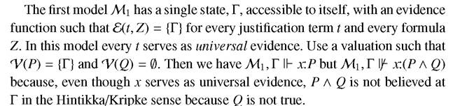
We now have that all theorems of J(CS) are valid in any Fitting model meeting constant specification CS. This means we can show unprovability variable). We construct two different countermodels for it. These are illustra­tive of some of the ideas behind the semantics. A formula t:X might fail at a possible world either because X is not believed there (it is false at some acces­sible world), or because t is not an appropriate reason for X. The two models illustrate these alternatives. To keep things uncluttered, we assume CS is the empty constant specification so we can ignore the role of justification constants in what follows.

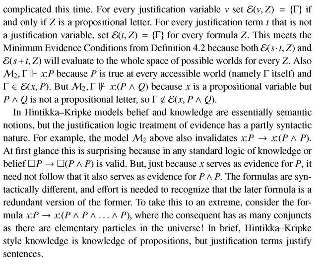
The second model M₂ again has a single state Γ accessible to itself. This time use the valuation V that assigns {Γ) to every propositional letter. It follows that both P andare true at Γ. The evidence function is somewhat more

4.3.2 LP

The first justification logic was LP, the Logic of Proofs.

Factivity is captured axiomatically with the scheme t:X → X. Modally, ?X → X corresponds to the semantic condition of reflexivity on Kripke models, and the same is the case for justification logics. It is easy to check that the Factivity scheme is valid in all Fitting models in which accessibility, R, is a reflexive relation. We use JT when referring to this logic, semantically or axiomatically (a completeness theorem will be shown soon, so there is no am­biguity between axiomatics and semantics here).

Positive Introspection modally is given by the axiom scheme ?X → ??X, which corresponds to a transitivity requirement on accessibility. The modal logic thus characterized axiomatically or semantically is called K4. For a justi­fication counterpart a unary operation symbol, !, is added to the language and

one adopts the axiom schemeFor Fitting models transitivity is

needed but is not enough. The justification analog of K4 is called J4, and se­mantically one requires that accessibility, R, be transitive on G, as in the modal case, and in addition we want the following.

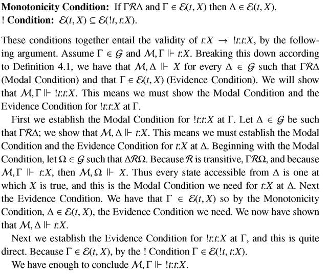
LP is the combination of JT and J4, and so is sometimes known as JT4. The name LP is retained for historical reasons. Semantically one assumes re­flexivity and transitivity of accessibility, the Monotonicity Condition, and the ! Condition.

4.3.3 K4³ and J4³

Modal K4³ and justification J4³ were introduced axiomatically in Section 2.7.1. Following Chellas (1980), in a modal model with possible worlds Γ and A and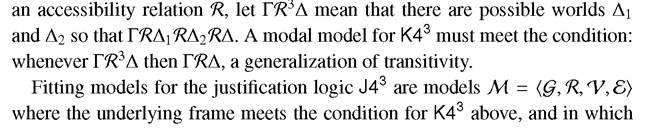

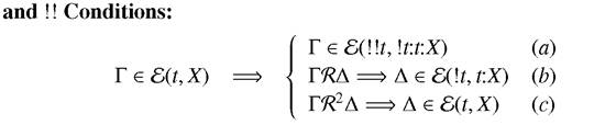
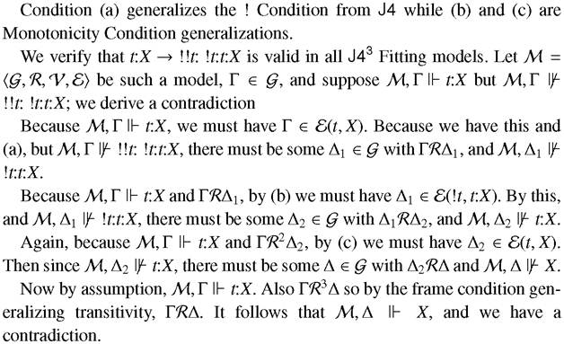
the evidence function meets the following conditions, generalizing from ! to !!.

4.3.4 S5 and JT45

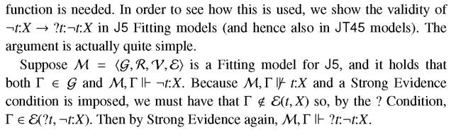
We have seen semantics for justification logics that are sublogics of LP, corre­sponding to sublogics of the modal logic S4. Historically, the first justification example that went beyond LP was JT45, corresponding to modal S5. It was discussed axiomatically in Section 2.7.2 and involves a negative introspection operator, “?”. There are three semantic conditions needed for this operator. First, the accessibility relation R should be symmetric, similar to S5 Kripke modal models. Here are the other two conditions, which have no modal analog.

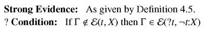
If these conditions are added to those for LP we have a semantics for the justification logic JT45. (If the conditions are added directly to J, the corre­sponding logic is called J5.) Notice that the ? Condition is stated with a nega­tive antecedent. Understanding how to handle this was a major breakthrough. Our formulation is from Rubtsova (2006a, b), with a similar approach given in Pacuit (2005, 2006). The most significant new thing is that a Strong Evidence

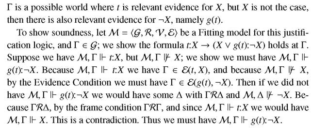
4.3.5 Sahlqvist Examples

We give semantic counterparts to the axiomatic presentation in Section 2.7.3.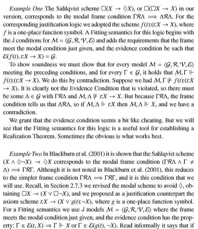

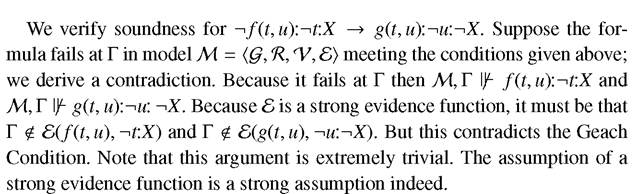
4.3.6 S4.2 and JT4.2

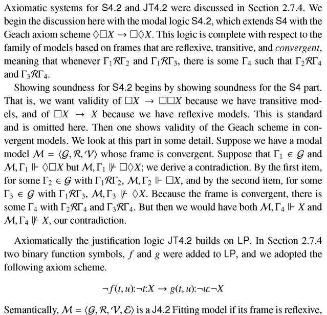
transitive, and convergent, as with S4.2, we have the LP requirements, the Monotonicity Condition, and the ! Condition from Section 4.3.2, E is a Strong Evidence function, Definition 4.5, and we have the following.

Geach Condition:

This material will be revisited in a much broader setting, in Section 8.2. A separate chapter is required because of both length and significance.

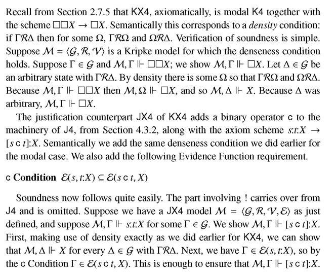
4.3.7 KX4 and JX4

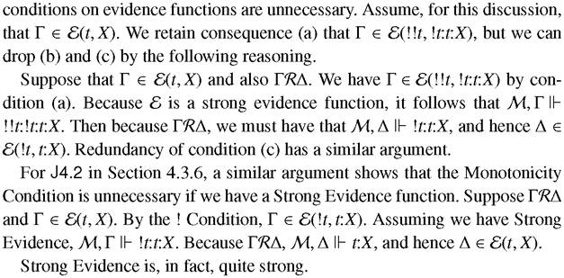
4.3.8 A Remark about Strong Evidence Functions

Imposing a strong evidence assumption can sometimes make other require­ments on a model redundant. For instance, if we restrict the semantics for J4³ from Section 4.3.3 to models with strong evidence functions, two of the three

4.4