A Benchmark Model of Technology Diffusion

18.2.1. A Model of Exogenous Growth. In the spirit of providing the main insights with the simplest possible models, let us return to the Solow growth model of Chapter 2. In particular, suppose that the world economy consists of J countries, indexed j = 1,...,J, each with access to an aggregate production function for producing the unique final good of the world economy,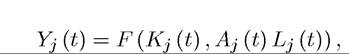

where Yj (t) is the output of this unique final good in country j at time t, and Kj (t) and Lj (t) are the capital stock and labor supply.

Using our usual approach, we can write income per capita as

is the effective capital-labor ratio of country j at time t.

We assume that time is continuous, that there is population growth at the constant rate nj ≥ 0 in country j, and that there is an exogenous saving rate equal to Sj ∈ (0,1) in country j and a depreciation rate of δ ≥ 0 for capital, so that the law of motion of capital for each country is given by

where

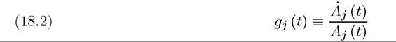
is the (endogenously-determined) growth rate of technology of country j at time t (see Exer­cise 18.1).

To start with, technology diffusion is modeled in a reduced-form way. Let us assume that

the world’s technology frontier, denoted by A (t), grows exogenously at the constant rate

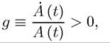
with an initial condition A (0) > 0. We refer to A (t) as the world technology or sometimes as

the “world technology frontier”. It encapsulates the maximal knowledge that any country can

following law of motion for each country’s technology:

where σj ∈ (0, ∞) and λj ∈ [0,g) for each j = 1,..., J (see Exercise 18.2). Equation (18.3) implies that each country absorbs world technology at some exogenous constant rate σj. We refer to this parameter as the technology absorption rate. In practice, absorption corresponds both to straightforward adoption of existing technologies and to adaptation of existing blue­prints to the conditions prevailing in a specific country, so that they can be used with the other technologies and practices in place. This parameter will vary across countries because of differences in their human capital or other investments (see below) and also because of 705

institutional or policy barriers affecting technology adoption. This parameter multiplies the difference A (t) — Aj (t), since it is this difference that remains to be absorbed by the country in question—if A (t) = Aj (t), there is nothing to absorb from the world technology frontier. Though natural, this formulation has important economic consequences. In particular, it implies that countries that are relatively “backward” in the sense of having a low Aj (t) com­pared to the frontier, will tend to grow faster, because they have more technology to absorb or or more room for catch-up.

Equation (18.3) also implies that technological progress can happen “locally” as well, that is building upon the knowledge stock of country j, Aj (t). The parameter λj captures the speed at which this happens. This equation therefore contains the two major forms of technological progress that a particular country can experience; absorption from the world technology frontier and local technological advances. Its functional form is adopted for sim­plicity.

Notice that (18.3) already sidesteps one of the major issues raised at the beginning of this chapter: it posits that despite the level of globalization the world has reached and the relatively free-flow of information among individuals across the globe, the process of technology transfer between countries is a slow one. The assumption that σj < ∞ imposes this feature. In particular, since σj < ∞, Aj (t) < A (t) will imply that Aj (t + ∆t) < A (t + ∆t), at least for ∆t > 0 and sufficiently small. Consequently, countries that have access to only a subset of the production techniques (blueprints) available in the world will not immediately acquire all of the knowledge that they do not currently have access to.

To proceed with the analysis of this model, let us define

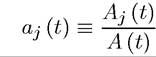
as an inverse measure of the proportional technology gap between country j in the world or alternatively as an inverse measure of country j’s distance to the frontier (distance to the world technology frontier), we can then write the above equation as (see Exercise 18.3):

(18.4)

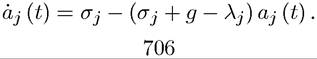
Clearly, the initial conditions A (0) > 0 and Aj (0) > 0 give a unique initial condition for the differential equation for aj, aj (0) ? Aj (0) /A (0) > 0.

Given the description of the environment above, the dynamics of the world income per capita levels and technology are determined by 2 J differential equations. For each j, we have one of (18.1) and one of (18.4). These equations characterize the state-state distribution of technology and income per capita in the world economy and its transitional dynamics. What makes the analysis of this world equilibrium relatively straightforward is the block recursiveness of the system of differential equations governing the behavior of income per capita and technology across countries. The law of motion of (18.4) for country j only depends on aj (t), so it can be solved without reference to the law of motion of kj (t) and to the law of motion of ∣kj∕ (t),αj∕ (t)}j∣j. Once (18.4) is solved, then (18.1) becomes a first-order nonautonomous differential equation in a single variable. The fact that it is nonautonomous is a consequence of the fact that it has gj (t) on the right-hand side, which can be determined as

Once we solve for the law of motion of aj (t), this is simply a function of time, making (18.1) a simple nonautonomous differential equation.

Let us start the analysis with the steady-state world equilibrium. A world equilibrium is defined as an allocationsuch that (18.1) and (18.4) are satisfied for

each j = 1,..., J and for all t, starting with the initial conditionsA steady­

state world equilibrium is then defined as a steady-state of this equilibrium process, i.e., an equilibrium withThe “steady-state equilibria” studied

in this chapter will exhibit constant growth, so I could have alternatively referred to them as balanced growth path equilibria.

Now imposing these steady-state conditions, we obtain the following straightforward proposition, which states that there exists a unique and globally stable steady-state equi­librium.

Proposition 18.1. In the above-described model, there exists a unique steady-state world equilibrium in which income per capita in all countries grows at the same rate g > 0. More­over, for each j = 1,..., J, we have

(18.5)

and kj is uniquely determined by

Proof. (Sketch) First solve (18.1) and (18.4) for each j = 1,...,J imposing the steady­state condition that kj (t) = aj (t) = 0. This yields a unique solution, establishing the uniqueness of the steady-state equilibrium. Then standard arguments show that the steady state aj of the differential equation for αj (t) is globally stable. Next using this result, the global stability of the steady state of the differential equation for kj (t) follows straightfor­wardly. Exercise 18.4 asks you to complete the details of this proof. ?

A number of features about this world equilibrium are noteworthy. First, we have a unique steady-state world equilibrium that is globally stable. This enables us to perform simple comparative static and comparative dynamic exercises (see Exercise 18.5). Second and most importantly, despite differences in saving rates and technology absorption rates across countries, income per capita in all economies grows at the same rate equal to the growth rate of the world technology frontier, g. Why is this? The technology adoption equation, (18.3), provides the answer to this question; the rate of technology diffusion (absorption) is higher when the gap between the world technology frontier in the technology level of a particular country is greater.

Does this imply that all countries will converge to the same level of income per capita? The answer is clearly no. Differences in saving rates and absorption rates translate into level differences (instead of growth rate differences) across countries. For example, a society with a low level of σj will initially grow less than others, until it is sufficiently behind the world technology frontier. At this point, it will also grow at the world rate, g. This discussion illustrates that it is precisely the endogenous technology gap between a country and the world frontier that ensures growth at the rate g for all countries. Thus societies that are unsuccessful in absorbing world technologies, those that impose barriers slowing technology diffusion (i.e., those with low σj) and those that are not sufficiently innovative in developing their own local technologies (i.e., those with low λj) will be poorer. Moreover, as in the baseline Solow model, those with low saving rates will also be poorer. These results are summarized in the following proposition.

Proof. See Exercise 18.7. ?

A particularly convenient—but also restrictive—feature of the equilibrium studied here is that even though there is technology diffusion and interdependence in this world equilibrium, there is no interaction among countries. Each country’s steady-state income per capita (and in fact path of income per capita) only depends on the behavior of the world technology frontier and its own parameters. Later in this chapter, we will see models in which there is more interaction between the decisions of individual countries.

18.2.2. Consumer Optimization. It is straightforward to incorporate consumer opti­mization into this benchmark model of technology transfer. In particular, let us now suppose that each country admits a representative household with preferences at time t = 0 given by

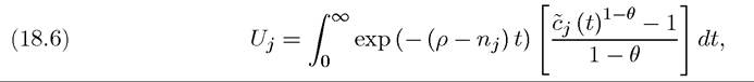
where Cj (t) ? Cj (t) /Lj (t) is per capita consumption in country j at time t and we have imposed that all countries have the same time discount rate, ρ. This latter feature is to simplify the discussion in the text, and Exercise 18.9 generalizes the results in this subsection to the world economy with different discount rates. This is an important generalization, since it highlights that a stable world income distribution does not depend on equal discount rates or asymptotically equal saving rates across countries.

As in the neoclassical growth model, the flow resource constraint facing the representative household can be written as

whereis consumption normalized by effective units

of labor. This equation now replaces (18.1) as the law of motion of effective capital-labor ratio of country j.

The world equilibrium and the steady-state world equilibrium are defined in a similar fashion, except that instead of a constant saving rate consumption sequences must now maximize the utility of the representative household in each country subject to their resource constraint. An analysis similar to that in Chapter 8 leads to the following proposition:

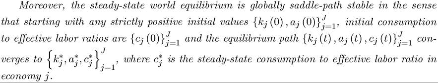
PROPOSITION 18.3. Consider the above-described model with consumer optimization with preferences given by (18.6) and suppose that ρ — nj > (1 — θ) g. Then, there exists a unique steady-state world equilibrium where for each j = 1,...,J, aj is given by (18.5) and kj is uniquely determined by

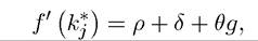
and consumption per capita in each country grows at the rate ä > 0.

Proof. (Sketch) We can first show that aj can be determined from the differential equa­tion in (18.4) without reference to any other variables and satisfies (18.5). The consumer Euler equations and the analysis of capital accumulation are the same analysis as in the baseline neoclassical growth model, taking into account that in steady state gj (t) = g. To complete the proof of the proposition, we need to show the stability of α^j, and then taking into account the behavior of gj (t), we must establish the saddle path stability of k^j using the same type of analysis as in Chapter 8—which is slightly more complicated here because the differential equation for capital accumulation is not autonomous. You are asked to complete these details in Exercise 18.8. ?

This proposition shows that all of the qualitative results of the benchmark model of technology diffusion apply irrespective of whether we assume constant saving rates or dynamic consumer maximization (as long as we ensure that the growth rate is not so high as to violate the transversality condition). Naturally, an equilibrium now corresponds not only to sequences of {kj (t),αj (t)} but also includes the time path of consumption per unit of effective labor, Cj (t). Consequently, the appropriate notion of stability is saddle-path stability, which the equilibrium in Proposition 18.3 satisfies.

18.2.3. The Role of Human Capital in Technology Diffusion. The model pre­sented above is in part inspired by a classic short paper by Richard Nelson and Edmund Phelps (1966). The Nelson-Phelps model focused on the role of human capital in technology adoption and is well known for having proposed a new role of human capital, different from those emphasized by Becker and Mincer. Recall that Becker and Mincer emphasized how human capital increases the productivity of the labor hours supplied by an individual. While this approach allows the effect of human capital to be different in different tasks, in most applications it is presumed that greater human capital translates into higher productivity in all or most tasks, with the set of productive tasks typically taken as given.

In contrast, Nelson and Phelps and Ted Schultz, who was at the same time writing on the role of human capital in technology adoption in agriculture, argued that the main role of human capital was not to increase productivity in existing tasks. Instead, human capital, they argued, was most important in facilitating the adoption of new technologies. In particular, Schultz viewed the agricultural world (or perhaps the less developed economies 710

more generally) to be in perpetual “disequilibrium” and argued that the main role of human capital was to enable individuals to deal with and adapt to situations of disequilibrium. Today, we would recognize what Schultz dubbed “disequilibrium” as an equilibrium of a dynamical system that is far from steady state (see Chapter 20 for a similar perspective). Thus his argument can be viewed as emphasizing the role of human capital in environments where certain key state variables, such as technology, are undergoing important changes. A similar argument was advanced by Nelson and Phelps’s famous short paper.

In terms of the model described above, the simplest way of capturing this argument is to posit that the parameter σj is a function of the human capital of the workforce. The greater is the human capital of the workforce, the higher is the absorption capacity of the economy. If so, high human capital societies will be richer because, as shown in Proposition

18.2, economies with higher σj have higher steady-state levels of income.

While this modification leaves the mathematical exposition of the model unchanged, the implications for how we view growth experiences of societies with different levels of human capital are potentially quite different than in the Becker-Mincer approach (or at the very least, than in the simplest version of the Becker-Mincer approach). The latter approach suggests that we can approximate the role of human capital in economic development by carefully accounting for its role in the aggregate production function. This, in turn, can be done by estimating individual returns to schooling and returns to other dimensions of human capital in the labor market. The Nelson-Phelps-Schultz view, on the other hand, suggests that the main role of human capital will be during periods of technological change and in the process of technology adoption. Thus it is the process of technological diffusion and adoption that makes human capital particularly valuable.

What is unclear in this view, however, is whether the contribution of human capital to national income through this particular role will be reflected in the wages of individual workers. For example, in the context of technology adoption decisions in agriculture, studied by Schultz, even though there is an important distinction between the role of human capital in facilitating technology absorption and its role in directly increasing productivity in existing tasks, both types of contributions will be reflected in an individual’s earnings—an individual with higher human capital, who successfully adopts new technologies, will become richer. If, on the other hand, the parameter σ_j in the above model is a function of human capital, this could be the result of each individual firm’s adoption decisions as a function of its own employees’ human capital or it might be working at the some higher level of aggregation than the firm, thus corresponding to externalities (recall Chapter 10). Therefore, while the Nelson-Phelps-Schultz view of human capital is conceptually different from the Becker-Mincer approach to human capital, whether this has major implications for empirically assessing the contribution of human capital to income differences across countries and over time depends

on whether the benefits created by human capital are internalized by firms and workers or whether they take the form of externalities. Consequently, as in the Becker-Mincer approach, if there are significant external effects, many of the empirical strategies discussed in Chapter 3 will understate the role of human capital. This discussion, however, emphasizes that were this to happen, it would be a consequence of human capital externalities, not a direct implication of the particular channel via which human capital affects productivity and growth. Therefore, if, as suggested by the discussion in Chapter 3, human capital externalities, except through global R&D effects, are limited, the Nelson-Phelps-Schultz view of human capital will not significantly change the conclusions about the contribution of human capital to differences in income differences across countries and over time.

18.2.4. Barriers to Technology Adoption. As discussed in Chapter 8, one of the main criticisms against the neoclassical growth model has been its inability to generate quantitatively large cross-country income per capita differences. Most economists view this as related to the fact that the basic neoclassical growth model does not provide an explana­tion for “technology differences”. The model in this section presents a reduced-form model of technology differences across countries, thus enables us to enrich the neoclassical growth model and the Solow model to incorporate technology differences. Nevertheless, such a theory will be useful only to the extent that the key parameters such as σj and λj can be mapped to reality. The previous subsection discussed ideas linking the parameter σj to human cap­ital. An alternative, emphasized by Parente and Prescott (1994), is to link σj to barriers to technology adoption. Parente and Prescott construct a variant of the neoclassical growth model in which investments affect technology absorption, and countries differ in terms of the “barriers” that they place on the path of firms in this process. In terms of the reduced-form model here, the Parente-Prescott mechanism can be captured by interpreting σj as a function of property rights institutions or other institutional or policy features.

This perspective is useful as it gives us a concrete way of thinking of the reasons why σ_j may vary across countries. Nevertheless, it is still unsatisfactory in two important respects. First, exactly how these institutions affect technology adoption is left as a black box. Sec­ond and more importantly, why some societies choose to create barriers against technology adoption while others do not is left unexplained. The models that combine technology dif­fusion with endogenous technology decisions, which will be presented in the next section, make some progress on the first point. In fact, Parente and Prescott constructed a model in which firms undertook investments to acquire technologies from the world technology frontier. Nevertheless, their model is closer to the neoclassical growth model than to the endogenous technology models presented in Part 4 of the book, because it does not feature investments in the creation or adoption of new technologies that can be identified with R&D decisions. Since 712

the endogenous technological change models we have seen above are more widely used and offer richer insights about the nature of technology, I will introduce endogenous technology adoption decisions in the context of these models. The question of why some societies block technology adoption will be the topic of Part 8 below.

18.3.