Technology Diffusion and Endogenous Growth
In the previous section, technology diffusion took place “exogenously,” in the sense that firms did not engage in R&D or investment type activities in order to improve their technologies.
In this section, we introduce these types of purposeful activities directed at improving technology. The material in this section therefore complements the models of technology diffusion of the previous section in the same way that endogenous technological change models complemented (and advanced upon) the neoclassical framework with exogenous technology. The section is separated into two parts. In the first, the world growth rate will be taken as exogenous, while it will be endogenized in the second part.18.3.1. Exogenous World Growth Rate. To keep the exposition as brief as possible, I will use the baseline endogenous technological change model with expanding machine variety and lab equipment specification as in Section 13.1 of Chapter 13 and I will frequently refer to the analysis there. Clearly, different versions of the endogenous technological change models could be used for the same purposes.
The aggregate production function of economy j = 1,...,J at time t is

where Lj is the aggregate labor input, which is assumed to be constant over time, Nj (t) denotes the different number of varieties of machines available to country j at time t, and Xj (v, t) is the total amount of machine type v used at time t. We continue to assume that x’s depreciate fully after use. As in Chapter 13, each variety in economy j is owned by a technology monopolist, which will sell machines embodying this technology at the profit maximizing (rental) price χj(v,t). This monopolist can produce each unit of the machine at a cost of ψ ? 1 — β units on the final good, where this normalization is again introduced to simplify the expressions.
Since there is no international trade, firms in country j can only use technologies supplied by technology monopolists in their country. This assumption introduces the potential differences in the knowledge stock available to different countries.
Each country admits a representative household with the same preferences as in (18.6), except that there is no population growth, i.e., nj = 0 for all j. New varieties are again produced by investment, and thus the resource constraint for each country at each point in time is

where Xj (t) is investment or spending on inputs at time t and Zj (t) is expenditure on technology adoption at time t, which may take the form of R&D or other expenditures, such as the purchase or rental of machines embodying new technologies. The parameter ζj is introduced as a potential source of differences in the cost of technology adoption across countries, which may result from institutional barriers against innovation as emphasized by Parente and Prescott (1994), from subsidies to R&D and to technology, or from other tax policies. As discussed in Section 8.9 in Chapter 8, many authors identify this parameter with tax distortions on investment-type activities and often proxy it with the relative price of investment to consumption goods. In the next chapter, we will see when this might be valid.
The main difference from the environment in Chapter 13 is in the innovation possibilities frontier,
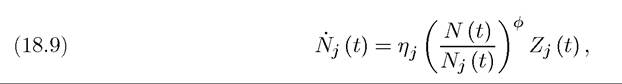
where ηj > 0 for all j, and φ > 0 and is common to all economies. This form of the innovation possibilities frontier captures the same basic idea as (18.3) in the previous section, but what matters is not the absolute gap in technology, but the proportional gap. This functional form is again adopted for simplicity. We assume that each economy starts with some initial technology stock Nj (0) > 0.
Finally, as noted above, for now we assume that the world technology frontier of varieties expands at an exogenous rate g > 0, i.e.,
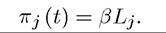
The analysis in Chapter 13 implies that the flow profits of a technology monopolist at time t in economy j is given by
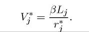
Suppose a steady-state (balanced growth path) equilibrium exists in which the interest rate is constant at some level Then the net present discounted value of a new machine is
If the steady state involves the same rate of growth in each country, then Nj (t) will also grow at the rate g, so that Nj (t) /N (t) will remain constant, say at some level ν). In that case, an additional unit of technology spending will create benefits equal to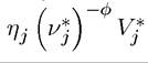 counterbalanced against the cost of ζj. Free-entry (with positive activity) then requires
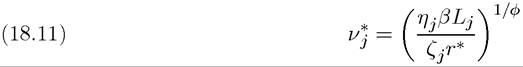
where I have also used the fact that given the preferences (18.6), equal growth rate across countries implies that the interest rate will be the same in all countries (and in fact it will be equal to r* = ρ + θg).
Since a higher Vj implies that country j is technologically more advanced and thus richer than others, equation (18.11) shows that societies with better innovation possibilities frontiers, as captured by the parameter ηj, and those with lower cost of R&D, corresponding to lower ζj, will be more advanced and richer. This equation also incorporates a scale effect as in the standard endogenous technological change models, so a country with a greater labor force will also be richer.
This is for the same reason as a greater labor force leads to faster growth in the baseline endogenous technological change model: a greater labor force creates more demand for machines, making R&D more profitable.This analysis leads to the following proposition:
PROPOSITION 18.4. Consider the model with endogenous technology adoption described in this section. Suppose that p > (1 — θ) g. Then there exists a unique steady-state world equilibrium in which relative technology levels are given by (18.11) and all countries grow at the same rate g > 0.
Moreover, this steady-state equilibrium is globally saddle-path stable, in the sense that starting with any strictly positive vector of initial conditions N (0) and (Ni (0),...,Nj (0)), the equilibrium path
Proof. (Sketch) First show that the specified steady-state equilibrium is the only steady state equilibrium in which all countries grow at the same rate. Then consider the value function of technology monopolist in each country as in Chapter 13 and show that the number of varieties in each countries must asymptotically grow at the rate g. Exercise 18.11 asks you to complete this proof. ?
This result and the preceding analysis therefore show that endogenizing investments in technology adoption leads to an equilibrium pattern similar to that we saw in the previous section. The main difference is that we can now pinpoint the factors that affect the rates of technology adoption and relate them to the profit incentives of firms. An explicit model of technology decisions also allows us to investigate how differences in the cost of investing in technology might affect cross-country differences in technology and income (see Exercise 18.12).
18.3.2. Endogenous Growth in the World. The model in the previous subsection was simplified by the fact that the world growth rate was exogenous. A more satisfactory model would derive the world growth rate from the technology adoption and R&D activities of each country.
Such models are typically more involved, because the degree of interaction among countries in the world equilibrium is now considerably greater. In addition, a certain amount of care needs to be taken so that the world economy grows at a constant endogenous rate, while there are still forces that ensure relatively similar growth rates across countries. Naturally, one may also wish to construct models in which countries grow at permanently different long run rates (see, for example, Exercise 13.8 in Chapter 13). The evidence we have seen in Chapter 1 suggests that such long-run growth differences are present when we look at the past 200 or 500 years, but there are more limited sustained growth rates differences over the past 60 years or so (implying only small changes in the postwar world income distribution). Thus whether one wants to have long-run growth rate differences across countries is a modeling choice—it partly depends on whether one thinks of a model with a long transition leading to the large income differences, or wishes to approximate the past 200 or 500 years as corresponding to “steady-state behavior”. Since such growth rates differences emerge straightforwardly in many models (including all of the endogenous technology models we have seen so far, see again Exercise 13.8), in this subsection we focus on forces that will keep countries growing at similar rates in the presence of endogenous technological change at the world level.The main difference from the model in the previous subsection is that we now replace the world growth equation, (18.10), which specified exogenous world growth at the rate g, with an equation that links the improvements in the world technology to technological improvements in each country. In particular, we assume the simplest way of aggregating the technologies of different countries, which is by taking their arithmetic average:
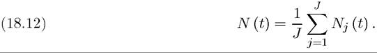
With this new equation, N (t) no longer corresponds to the “world technology frontier”.
Instead, it represents average technology in the world, and as long as there are some differences across countries, it will naturally be the case that Nj (t) > N (t) for at least some j. Nevertheless, having the world technology an average of the technology of each country is a natural generalization of the ideas presented so far in this chapter. One disadvantage of this formulation is that it implies that the contribution of each country to the world technology is the same. Exercise 18.18 discusses alternative ways of aggregating individual country technologies into a world technology term and shows that the qualitative results here do not depend on the specification in (18.12). Besides equation (18.12), we assume that all the other equations from the previous subsection continue to hold.The main result of this section is that the pattern of cross-country growth will be similar to that in the previous subsection, but now the growth rate of the world economy, g, will be endogenous, resulting from the investments in technologies made by firms in each country. In particular, suppose that there exists a steady-state world equilibrium in which each country grows at the rate g. Then, (18.12) implies that the world technology index, N (t), will also grow at the same rate g. Now, as in the previous subsection, the net present discounted value of a new machine in country j is
and the no-arbitrage condition in R&D investments implies that, for given g, each country j's relative technology, νj, should satisfy (18.11). However, now dividing both sides of equation (18.12) by N (t) implies that the steady-state world equilibrium must satisfy:
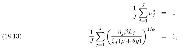
where the second line uses the definition of νj from (18.11) and substitutes for the common interest rate r* as a function of the world growth rate. The only unknown in equation (18.13) is g. Moreover, the left-hand side is clearly strictly decreasing in g, so this equation can be satisfied for at most one value of g, say g*. A well-behaved world equilibrium would require the growth rates to be positive and not so high as to violate the transversality condition. The following condition is necessary and sufficient for the world growth rate to be positive:

Moreover, by usual arguments, when this condition is satisfied, there will exist a unique g* > 0 that will satisfy (18.13) (if this condition were violated, (18.13) would not hold, and we would have g = 0 as the world growth rate). Therefore, the following proposition follows:
Proposition 18.5. Suppose that (18.14) holds and that the solution g* to (18.13) satisfies p > (1 — θ) g*. Then there exists a unique steady-state world equilibrium in which growth at the world level is given by g* and all countries grow at this common rate. This growth rate is endogenous and is determined by the technologies and policies of each country. In particular, a higher ηj or Lj or a lower ζj for any country j = 1,..., J increases the world growth rate.
Proof. See Exercise 18.15. ?
A number of features about this equilibrium are noteworthy. First, taking the world growth rate as given, the structure of the equilibrium is very similar to that in Proposition
18.4. Thus the fact that all countries grow at the same rate and that differences in the innovation possibilities frontier, ηj, the size the labor force, Lj, and the extent of potential distortions in technology investments, ζj, translate into level differences across countries has exactly the same intuition as in that proposition. What is more interesting is that essentially the same model as in the previous subsection now gives us an “endogenous” growth rate for the world economy. In particular, while growth for each country appears “exogenous” in the sense that, each country accumulates towards a world-determined growth rate, the growth rate of the world economy is endogenous and results from the investments of the firms in each country. As such, the current model provides a more satisfactory framework for the analysis of the process of world growth than both the purely exogenous growth models and the purely endogenous growth models. In the current model, technological progress and economic growth are the outcome of investments by all countries in the world, but there are sufficiently powerful forces in the world economy, here working through technological spillovers that pull relatively backward countries towards the world average, ensuring equal long-run growth rates for all countries in the long run. Naturally, equal growth rates are still consistent with quite large level differences across countries (see Exercise 18.12).
Proposition 18.5 used a number of simplifying assumptions. First, each country was assumed to have the same discount rate. This was only for simplicity, and Exercise 18.16 considers the case in which countries differ according to their discount rates. Second, the proposition only describes the steady-state equilibrium. Transitional dynamics are now more complicated, since the “block recursiveness” of the dynamical system is lost. The differential equations describing the equilibrium path for all countries need to be analyzed together. Nevertheless, local stability of the steady-state world equilibrium can be established, and this is analyzed in Exercise 18.15.
18.4.