Dynamic Effects of Fiscal Policy in the Blanchard-Weil Model

We next examine the impact of fiscal policy in the Blanchard-Weil OLG model. The basic model was analyzed in chapter 5. Here, we introduce the government to this model.

6.3.1 The Blanchard-Weil Model with Government Expenditure and Debt

The Blanchard-Weil model with constant government expenditure , and government debt , per efficiency unit of labor, as implied by (6.13) and (6.14), is described by the following two differential equations:

All variables are expressed per efficiency unit of labor.

The only difference from the Ramsey model of section 6.2 is in equation (6.18) for the adjustment of private consumption. Because new entrants to the economy do not have accumulated savings in the form of either capital k or government bonds , the change in private consumption depends negatively on k + multiplied by the product of the proportion of new entrants in total population n and their propensity ρ to consume out of wealth.

6.3.2 Government Debt, Taxes, and Redistribution across Generations

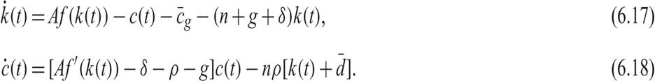
The behavior of the model is analyzed in figure 6.2. The balanced growth path is at point E, where both (6.17) and (6.18) are satisfied for constant consumption and capital per efficiency unit of labor. A unique saddle path leads to the balanced growth path. One can see that E implies lower consumption and capital per efficiency unit of labor than the corresponding representative household model at point R. Point R is the balanced growth path of a corresponding economy with n = 0 in (6.18), which is the balanced growth path of a representative household economy.

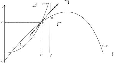
Figure 6.2 Primary government expenditure and debt in the Blanchard-Weil model.

With the help of the phase diagram in figure 6.3, one can easily show that a previously unanticipated permanent one-off increase in government debt leads to a reduction of both steady state capital and steady state private consumption. When government debt rises in a one-off fashion, consumption rises to point E₀ on the new saddle path, as current generations treat their higher bond holdings as an increase in their wealth. This initiates a process of decumulation of capital and declining private consumption, which leads the economy toward the new balanced growth path at E^′.

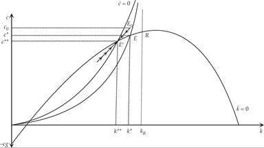
Figure 6.3 An increase in government debt in the Blanchard-Weil model.

With the help of figure 6.4, one can show that a permanent increase in primary government expenditure financed by a rise in autonomous taxes also leads to lower steady state capital and private consumption. When the increase in government expenditure occurs, private consumption falls, as current generations react to the increase in the present value of their taxes. However, the anticipated increase in the present value of taxes for current generations is lower than the increase in the present value of primary government expenditure. This is because part of the future tax burden will be shouldered by future generations. Thus, private consumption falls by less than the increase in primary government expenditure, and total savings fall relative to equilibrium investment. This starts a process of capital decumulation and declining consumption on the new saddle path, which leads the economy to a new balanced growth path with lower steady state capital, output, and consumption per effective unit of labor.

Figure 6.4 An increase in primary government expenditure in the Blanchard-Weil model.

As one can deduce from this analysis, in an OLG model, both the level of government debt and taxes and the primary government expenditure affect the balanced growth path. Ricardian equivalence does not hold, because current generations know that part of the increase in the present value of taxes required to finance an increase in government debt (or primary government expenditure) will be borne by future generations. Thus, total savings and capital accumulation are affected, as government debt and expenditure policies essentially redistribute wealth across generations.³

Exercise 6.1 Introduce the government budget constraint in the simplified Diamond model of chapter 5 with logarithmic preferences and a Cobb-Douglas production function. Assume that taxes are lump sum and are levied on the young.

6.3.3 Dynamic Simulations of Fiscal Policy in a Calibrated Blanchard-Weil Model

The fiscal policies we have considered so far are restricted to one-off permanent increases in either primary government expenditure or government debt, per efficiency unit of labor. This has allowed us to eliminate the dynamics of government debt accumulation and keep our model simple and analytically tractable (in that it consists of two differential equations, with one state and one control variable).

We shall now examine a more realistic description of fiscal policy in the Blanchard-Weil model, where the government chooses a level of primary government expenditure and autonomous taxes. The model then allows taxes and government debt to adjust gradually, in a way that satisfies the government budget constraint. Thus, we again assume that the government has a fixed target for primary government expenditure:

However, let us now assume that the government changes taxes to stabilize government debt per efficiency unit of labor only gradually and not immediately, as in equation (6.14). To do this, it uses a tax-smoothing policy of the form

where , and ψ > r_E − n − g > 0.

Substituting (6.19) and (6.20) in (6.12), government debt per efficiency unit of labor evolves according to

Three parameters now describe fiscal policy: , primary government expenditure per efficiency unit of labor; , autonomous taxes; and ψ, the responsiveness of taxes to government debt.

The differential equation (6.21) will be stable if the responsiveness of taxes to government debt ψ is higher than r(t) − n − g, which, as we have assumed, will certainly apply in the steady state.

Let us now consider the simulation of a calibrated version of the Blanchard-Weil model, assuming a Cobb-Douglas production function of the form Ak^α, as in the previous simulations. We thus consider the simulation of a discrete time version of the model described by (6.17) and (6.18), using a Cobb-Douglas production function; the marginal productivity conditions for the determination of real wages and the real interest rate; and the assumptions about fiscal policies embodied in (6.19), (6.20), and (6.21).

The parameter values in the simulations are as follows: A = 1, α = 0.333, ρ = 0.02, θ = 1, n = 0.01, g = 0.02, δ = 0.03. These values are the same as the ones used in previous simulations, such as the simulations discussed in chapters 3, 4, and 5. As for the parameters of fiscal policy, let us assume that = 0.5, = 0.45, and ψ = 0.075.⁵

We consider three alternative fiscal policy shocks. First, a 10% tax-financed increase in primary government expenditure (from 0.5 to 0.55; see figure 6.5). This policy does not result in an increase in government debt. Second, a 10% debt-financed increase in primary government expenditure (from 0.5 to 0.55; see figure 6.6). This policy results in an increase in government debt but also eventually in taxes, through the induced stabilizing reaction of taxes to the rise in government debt. Third, a debt-financed cut in autonomous taxes by 0.05 (see figure 6.7). This last shock amounts to a temporary tax cut equivalent to a 10% increase in governement expenditure. This tax reduction causes an increase in government debt and eventually, by means of equation (6.20), causes an increase in total taxes, because of the induced stabilizing reaction of taxes to the rise in government debt.

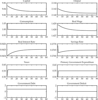
Figure 6.5 A tax-financed increase of primary government expenditure in the calibrated Blanchard-Weil model.

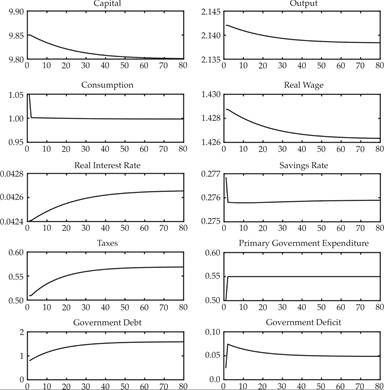
Figure 6.6 A debt-financed increase of primary government expenditure in the calibrated Blanchard-Weil model.

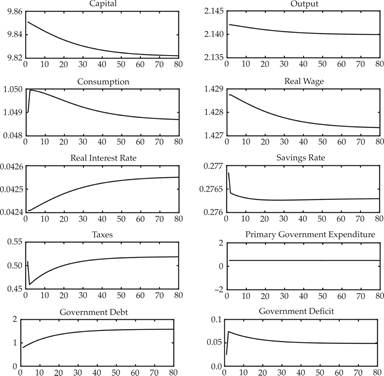
Figure 6.7 A debt-financed tax cut in the calibrated Blanchard-Weil model.

Figure 6.5 depicts the effects of a permanent tax-financed increase in primary government expenditure by 0.05 (10% of its original level). This increase reduces private consumption expenditure immediately because of the increase in autonomous taxes. However, as part of the future autonomous taxes will be paid by future generations, the reduction of private consumption by current generations is lower than the increase in primary government expenditure, and total savings fall. This starts a process of decumulation of capital that leads the economy to a new steady state, with lower capital, output, private consumption, and real wages per efficiency unit of labor, as well as a higher real interest rate.

However, note that the effects of an tax-financed increase in primary government expenditure on steady state nonfiscal real variables are extremely small. A 10% increase in real primary government expenditure (such as the one we have considered) reduces steady state real per capita output (and real wages) by only 0.07% and increases the steady state real interest rate by only 0.01 percentage points (i.e., from 4.24% to 4.25%). The steady state aggregate savings rate is reduced from 27.7% to 27.6%, again a very small decline.

Figure 6.6 depicts the effects of a debt-financed increase in primary government expenditure by 0.05 (10% of its original level). This increase also reduces private consumption expenditure immediately, because of the anticipated future increase in taxes that will be required for debt to be eventually stabilized. However, as part of the future taxes will be paid by future generations, the reduction of private consumption by current generations is lower than the increase in primary government expenditure, and total savings fall. This starts a process of decumulation of capital that leads the economy to a new steady state with lower capital, output, private consumption, and real wages per efficiency unit of labor, as well as a higher real interest rate. Government debt is also increasing in the process and ends up at more than double its initial level.

Again, note that the effects of a debt-financed increase in primary government expenditure on nonfiscal steady state real variables are extremely small, although larger than for a tax-financed increase. A 10% increase in real primary government expenditure (such as the one we have considered) reduces steady state real per capita output (and real wages) by only 0.17% and increases the steady state real interest rate by only 0.03 percentage points (i.e., from 4.24% to 4.27%). The steady state aggregate savings rate is reduced from 27.7% to 27.6%, again a very small decline. However, the steady state debt to GDP ratio more than doubles, rising from 79% of GDP to 159% of GDP. Thus, although the real effects of a debt-financed increase in primary government expenditure on per capita real output and the real interest rate are almost three times as high as the effect of an equivalent tax-financed increase, they remain extremely small.

Finally, figure 6.7 depicts the effects of debt-financed cut in autonomous taxes by 0.05 (10% of the level of primary government expenditure). This cut increases private consumption expenditure immediately, because current generations anticipate that the future increases in taxes that will be required for the debt to be stabilized will be paid in part by future generations. The increase in private consumption and the associated reduction in savings start a process of decumulation of capital that leads the economy to a new steady state, with lower capital, output, private consumption, and real wages per efficiency unit of labor, as well as a higher real interest rate. Government debt is also increasing in the process and ends up being more than double its initial level.

The effects of a debt-financed cut in autonomous taxes on nonfiscal real variables are also extremely small. A 10% reduction in autonomous taxes reduces steady state real per capita output (and real wages) by only 0.10% and increases the steady state real interest rate by only 0.02 percentage points (from 4.24% to 4.26%). The steady state aggregate savings rate is reduced from 27.7% to 27.6%, again a very small decline. Thus, the real effects of a debt-financed cut in autonomous taxes are extremely small—even smaller than a debt-financed rise in primary government expenditure. However, the steady state debt to GDP ratio more than doubles, rising from 79% of GDP to 159% of GDP.

The results of these simulations are extremely informative. They suggest that although Ricardian equivalence does not hold in OLG models, the deviations from Ricardian equivalence imply very small real effects on steady state real variables (such as the savings rate, or per capita real output, real wages, and real interest rates).

This observation should not be very surprising, as the non-Ricardian effects in OLG models depend on the product of two quantitatively small parameters: population growth (which is assumed to take place through the entry of new generations) and the pure rate of time preference (which determines the proportion of total assets consumed by households). With a population growth rate of 1% per year and a pure rate of time preference of 2% per year (as assumed in the simulations), the product of the two is only 0.02%, a very small number indeed.⁶

6.4