Ricardian Equivalence and the Ramsey Model

Let us now introduce the government in the Ramsey model of a representative household that we analyzed in chapter 4. Assume that the government engages in primary spending and finances this primary spending through a combination of debt and taxes that satisfies the government budget constraint (6.4).

6.2.1 Ricardian Equivalence between Government Debt and Taxes

When there are taxes and a stock of government debt, the intertemporal budget constraint of the representative household implies that the present value of its (private) consumption cannot exceed the value of its current assets (capital plus government bonds) plus the present value of its disposable labor income (i.e., its after-tax labor income). Thus, the intertemporal budget constraint of the representative household is given by

where C(t) is the real consumption of the representative household at time t; W(t) is its real labor income at time t; K(0) is its initial stock of capital; and D(0) the initial stock of government bonds, held as assets by the representative household. Expression (6.7) can be rewritten as

Assume that the government satisfies its intertemporal budget constraint (6.4) exactly, in the sense that the present value of future taxes minus its initial debt is equal to the present value of primary government expenditure. Substituting (6.4) in (6.8), we get

which suggests that we can express the intertemporal budget constraint of the representative household as a function of the present value of primary government expenditure without any reference to the method of financing it.

Because the path of tax revenue or the original debt does not affect the budget constraint or the preferences of the representative household, the path of tax revenue or the level of government debt cannot possibly affect private consumption. Thus, (6.9) leads us to conclude that the only aspect that matters for the course of private consumption is the present value of primary government expenditure and not the method of financing it (i.e., through taxes or government debt).

This result is demonstrated in an important paper by Barro [1974], and it has since been known as Ricardian equivalence between debt and taxes. It is a result we also demonstrated for the two-period model of chapter 2.²

Government bond holdings by the representative household are not considered a net addition to its wealth, as the representative household realizes that its bond holdings will be financed by future taxes of equal present value.

6.2.2 Government Expenditure, Taxes, and Debt in the Ramsey Model

We can analyze the Ricardian equivalence result in a different way, by introducing the government in the full Ramsey model of chapter 4.

The Euler equation for consumption is not affected by introducing the government. It is given by

The capital accumulation equation takes the form

Total savings in (6.11) are now defined by the difference between total income and total consumption (private and public).

Finally, government debt evolves according to (6.1). Expressing government debt accumulation per efficiency unit of labor, we get

where c is private consumption, k the stock of capital, d the stock of government debt, c_g primary government expenditure, and τ taxes, all defined in real terms per efficiency unit of labor. In (6.12), the marginal productivity condition r(t) = Af′(k(t)) − δ has been used to substitute out for the real interest rate.

Let us examine policies with exogenous and constant primary government expenditure per efficiency unit of labor. Thus, assume that the government stabilizes primary government expenditure at

where is a constant target level of primary government expenditure (per efficiency unit of labor).

Further assume that the government uses taxes to stabilize government debt per efficiency unit of labor. From (6.12) and (6.13), this requires a tax policy of the form

where is a constant target level of government debt (per efficiency unit of labor). Equation (6.14) implies that taxes are equal to the level of primary government expenditure plus the part of the interest payments on government debt that must be financed by taxes, so that debt per efficiency unit of labor remains constant.

In the representative household model, the real interest rate converges to ρ + θg, so that taxes per efficiency unit of labor converge to the steady state value

Steady state taxes are equal to the level of primary government expenditure plus the part of the interest payments on government debt that must be financed by taxes, so that debt per efficiency unit of labor remains constant.

The evolution of capital and savings per efficiency unit of labor is described by the Euler equation for consumption (6.10) and the capital accumulation equation (6.11) for constant primary government expenditure per efficiency unit of labor, as in (6.13). Thus, the capital accumulation equation is given by

The balanced growth path and the dynamic adjustment path are presented in figure 6.1. For comparison, the figure also shows the equilibrium for zero primary government expenditure, which lies above E. It is clear from figure 6.1 that primary government expenditure only leads to an equal reduction in private consumption without any other effect on real variables. An increase in primary government expenditure causes an equal reduction in private consumption due to the increase in the present value of future taxes (which reduces the present value of disposable labor income of the representative household). The stock of government debt has no effect at all on private consumption, because the method of financing government expenditure does not affect the intertemporal budget constraint of the representative household.

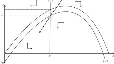
Figure 6.1 Primary government expenditure in the Ramsey model.

If the economy is out of steady state, the adjustment takes place along the unique saddle path that leads to the steady state.

In conclusion, in the representative household model, primary government expenditure, government debt, and taxes do not affect aggregate savings and the balanced growth path, nor do they change the adjustment path toward the steady state. Primary government expenditure crowds out an equal amount of private consumption and has no other effects on either the balanced growth path or the adjustment path. Aggregate savings and the accumulation of capital are not affected by the level of primary government expenditure, in either the short or the long run. In addition, the method of financing government expenditure (i.e., the steady state level of government debt per efficiency unit of labor) has no effect on either the steady state or the adjustment path. These Ricardian equivalence results were also proven for the two-period representative household model in chapter 2.

6.3