Labor Market Equilibrium

Identify factors that affect labor market equilibrium.

FIGURE 3.9

Labor market equilibrium

The quantity of labor demanded equals the quantity of labor sup­plied at point E.

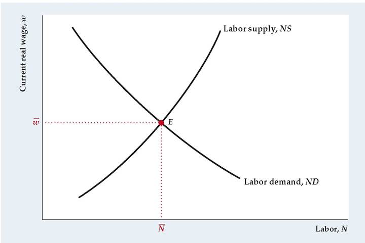
doesn't shift. Equilibrium in the labor market moves from point A to point B. Thus the model predicts that a temporary supply shock will lower both the current real wage (from W ₁ to W ₂) and the full-employment level of employment (from N₁ to N ₂).

The classical supply-demand model of the labor market has the virtue of sim­plicity and is quite useful for studying how economic disturbances or changes in economic policy affect employment and the real wage. However, a significant

FIGURE 3.10

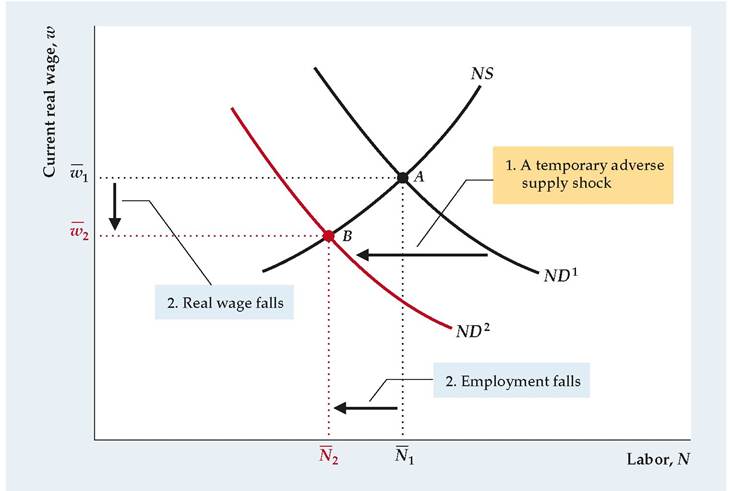
drawback of this basic model is that it cannot be used to study unemployment. Because it assumes that any worker who wants to work at the equilibrium real wage can find a job, the model implies zero unemployment, which never occurs. We discuss unemployment later in this chapter, but in the meantime we will con­tinue to use the classical supply-demand model of the labor market.

Full-Employment Output

By combining labor market equilibrium and the production function, we can deter­mine the amount of output that firms want to supply. Full-employment output, Y, sometimes called potential output, is the level of output that firms in the economy supply when wages and prices have fully adjusted. Equivalently, full-employment output is the level ofoutput supplied when aggregate employment equals its full­employment level, N.

Equation (3.4) shows that, for constant capital stock, K, full-employment out­put is determined by two general factors: the full-employment level of employ­ment,, and the production function relating output to employment.

Anything that changes either the full-employment level of employment, N, or the production function will change full-employment output, Y. For example, a temporary adverse supply shock that reduces the MPN (Fig. 3.10) works in two distinct ways to lower full-employment output:

1. The adverse supply shock lowers output directly, by reducing the quantity of out­put that can be produced with any fixed amounts of capital and labor. This direct effect can be thought of as a reduction in the productivity measure A in Eq. (3.4).

2. The adverse supply shock reduces the demand for labor and thus lowers the full-employment level of employment N, as Fig. 3.10 shows. A reduction in N also reduces full-employment output, Y, as Eq. (3.4) confirms.

Application

Output, Employment, and the Real Wage During Oil Price Shocks

Among the most severe supply shocks hitting the U.S. and world economies since World War II were sharp increases in the prices of oil and other energy products. Figure 3.11 shows how the price of energy paid by firms, measured relative to the GDP deflator (the general price level of all output), varied during the period 1960-2017. Three adverse oil price shocks stand out: one in 1973-1974, when the Organization of Petroleum Exporting Countries (OPEC) first imposed an oil embargo and then greatly increased crude oil prices; a second in 1979-1980, after the Iranian revolution disrupted oil supplies; and a third in 2003-2008, when surging demand for oil by large rapidly developing countries such as China and India, combined with weak supply (because of insufficient production capacity, hurricanes that damaged Gulf of Mexico production, and geopolitical concerns in the Middle

(continued)

FIGURE 3.11

Relative price of energy, 1960-2021

The figure shows the producer price index of fuels and related prod­ucts and power (an index of energy prices paid by producers) relative to the GDP deflator.

Sources: Bureau of Economic Analysis, downloaded from FRED database at fred.stlouisfed. org. Producer price index for fuels and related products and power: FRED series PPIENG; GDP deflator: FRED series GDPDEF. Data were scaled so that the relative price of energy equals 100 in year 2000.

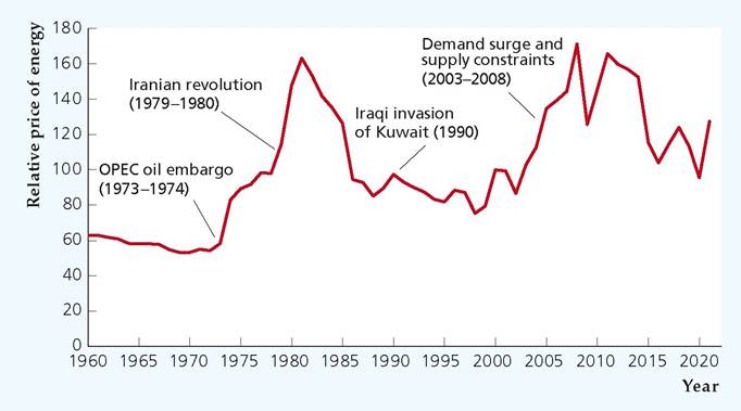
East, Russia, Venezuela, and Nigeria) caused the price of oil to rise sharply. The 1979-1980 oil price shock turned out to be temporary, as energy prices subse­quently fell. The increase in oil prices following Iraq's invasion of Kuwait in August 1990 had less of an impact on overall energy prices than the three oil price shocks mentioned above and thus doesn't appear as much more than a blip in Fig. 3.11.

When a reduction or disruption in the supply of oil causes energy prices to rise, firms cut back on energy use, implying that less output is produced at any particular levels of capital and labor, which is an adverse supply shock. How large is the effect on GDP from an oil price shock? It is difficult to disentangle everything else going on in the economy when such a shock occurs and the out­come depends on the government's policy response. But empirical research sug­gests that an increase of 10% in the price of oil reduces GDP by about 0.4 per­centage points.^[47] Thus the 96% increase in oil prices from 2002 to 2008 led GDP to be about 3.8% lower than it would have been in the absence of the increase in oil prices.

Our analysis predicts that an adverse supply shock will lower labor demand, reducing employment and the real wage, as well as reducing the supply of output. In fact, the economy went into recession, with negative GDP growth, following the increases in oil prices resulting from restrictions in the supply of oil in 1973-1974, 1979-1980, and 1990. In each case, employment and the real wage fell. Care must be taken in interpreting these results because macroeco­nomic policies and other factors were changing at the same time; however, our model appears to account for the response of the economy to these major oil price increases.

3.5