Political Institutions and Growth-Enhancing Policies
In this section, I consider the canonical Cobb-Douglas model analyzed in subsection 22.2.4 (and then used again in Sections 22.3 and 22.4 of the previous chapter). In that chapter, this model was analyzed under the assumption that the group of producers which I referred to as the “elite” were in power.
I showed how the political equilibrium in this case can lead to various different forms of non-growth-enhancing policies. I will now briefly discuss the equilibrium in the same environment when the middle class or the workers are in power and then contrast the resulting allocations.23.2.1. The Dictatorship of the Middle Class Versus the Dictatorship of the Elite. First, let us suppose that the middle class hold political power, so that we have the dictatorship of the middle class instead of the dictatorship of the elites in the previous chapter. The situation is entirely symmetric to that in the previous chapter with the middle class and the elite having exchanged places. In particular, the analysis leading to Proposition 22.6 immediately yields the following result.
Proposition 23.1. Consider the environment of subsection 22.2.f with Cobb-Douglas technology, but the middle class instead of the elite holding political power. Suppose that Condition 22.1 holds, φ > 0, and

Then the unique Markov Perfect Political Economy Equilibrium features τm (t) = O and
Proof. See Exercise 23.2. ?
The notable feature about this equilibrium is the strong parallel to Proposition 22.6.
The equilibria under elite control and middle class control are identical, except that the two groups have switched places. We therefore have an example of political institutions having a real effect on both the types of economic policies and economic institutions in place, and on the allocation of resources; in the elite-controlled society, the middle class are taxed both to create revenues for the elite and to reduce their labor demand.
In the middle class dominated society, the competing group of producers that are out of political power are the “elite” (even though the name “elite” has the connotation of political power). So now the elite are taxed to generate tax revenue and to create more favorable labor market conditions for the middle class. The contrast between the elite dominated and the middle class dominated politics approximates certain well-known historical episodes. For example, in the context of the historical development of European societies, political power was first in the hands of landowners, who exercised it to keep labor tied to land and to reduce the power and the profitability of merchants and early industrialists (capitalists). In many cases, these policies favoring landowners were detrimental to economic growth. Nevertheless, with economic changes and the constitutional revolutions taking place in the late medieval period, power shifted away from landowning aristocracies towards the merchants and Lists, and it was their turn to adopt policies favorable to their own economic interests and costly for landowners. The repeal of the Corn Law in 1846 illustrates this point, even though the conflict between landowners and capitalists was probably weakest in England because many members 1030of the gentry and the previous landowning class had already transitioned into commercial agriculture and other industrial activities. Nevertheless, there were intense political debates surrounding the Corn Law, with landowners supporting the tariffs imposed by the law, which kept the price of their produce high, and industrialists opposing it so that the implicit tax on their inputs, especially labor, would be removed with the import of cheaper corn from abroad.
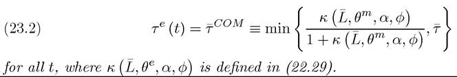
So which one of these two sets of political institutions—the dictatorship of the middle class or the dictatorship of the elite—is better? The answer is that they cannot be compared easily. First, as already emphasized in the previous chapter, the equilibrium considered in Section 22.3 was already Pareto optimal; starting from the allocation there, it is not possible to make any member of the society better off without making the elite worse off.
In the same way, the current allocation of resources is Pareto optimal, but it has picked a different point along the Pareto frontier—a point that favors middle-class agents instead of the elite. However, in the previous chapter we also emphasized that Pareto optimality may be too weak a concept for a useful analysis of the effect of institutions on economic growth, since two allocations that are Pareto optimal may involve significantly different growth rates. And yet, when we compare the growth rates under these two different political regimes, we also find that there is no straightforward ranking. Either of these two societies may achieve a higher level of income per capita. Which one does so depends on which group has more productive investment opportunities. When the middle class has the more productive investment opportunities, a society in which the elite are in power will create significant distortions. In contrast, if the elite have more profitable and socially beneficial production opportunities, then having political power vested with the elite is more beneficial for economic performance than the dictatorship of the middle class.The following proposition illustrates a particularly simple case of this result.
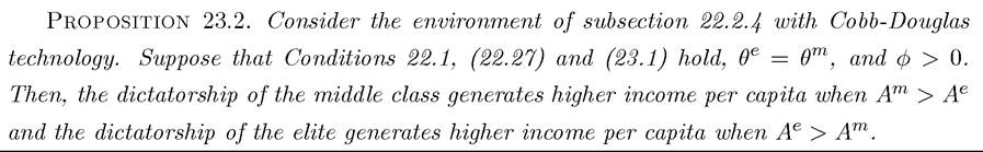
Proof. See Exercise 23.3. ?
This proposition therefore gives a simple example of a situation whereby which political institutions will lead to better economic performance (in terms of income per capita) depends on whether the group that is more productive also holds political power. When political power and economic power are decoupled, there is greater inefficiency. An immediate implication of this result is that it is difficult to think of “efficient political institutions” without considering the self-interested objectives of those who hold and wield political power 1031
and without fully analyzing how their productivity and their economic activities compare to those of others.
Naturally, one can dream of political institutions that will outperform both the elite dominated politics of the previous chapter and the middle class dominated politics of this chapter. For example, we can think of a set of political institutions that constitutionally force all taxes to be equal to zero—so that in the context of the simple model we are focusing on here, there are no distortionary policies. In this environment, this alternative arrangement will outperform both elite dominated and middle class dominated polities. However, such political institutions are not realistic. First, there are numerous reasons why societies need to raise taxes, for example, they need to finance productivity-enhancing public goods as in the model of Section 22.8 in the previous chapter, and they also need to engage in some amount of redistribution to ensure a safety net to their citizens. Once we allow for positive taxes, then the social groups or the politicians that are in power can also misuse these tax revenues and the associated fiscal instruments. Second, constitutional limits on taxes are difficult to enforce. Once a particular group is in power and has the capability to dictate policies, there is no easy way of preventing them to rewrite the constitution as has been the practice in many countries over the last two centuries. This discussion indicates that we can think of “ideal political institutions” that may prevent the distortions of simpler institutions that vest power with a particular group of individuals, but such political institutions are difficult to create, implement and maintain. Most likely, they are not even feasible. And this implies that the choice of political institutions in practice will be between arrangements that will create different types of distortions and different winners and losers.23.2.2. Democracy or Dictatorship of the Workers? The previous subsection contrasted the dictatorship of the middle class to the dictatorship of the elite. A third possibility is to have a more democratic political system in which the majority decides policies.
Since in realistic scenarios, the workers will outnumber both the elite and the middle class, this means the choice of policies that favor the economic interests of the workers (who have so far been passive in this model, simply supplying their labor at the equilibrium wage rate) will be implemented. While such a system does resemble democracy in some ways, it can also be viewed as a dictatorship of the workers, since it will now be the workers who will dictate policies, in the same way that the elite or the middle class dictated policies under their own dictatorship.[53] [54] This emphasizes once more that different political institutions will create different winners and losers depending on which group has more political power.The analysis is again straightforward, though the nature of the political equilibrium does depend even more strongly on whether or not Condition 22.1 holds (i.e., whether there is excess supply or not). The following proposition summarizes the equilibrium choices of policies by the workers when they monopolize political power.
Proposition 23.3. Consider the environment of subsection 22.2.f with Cobb-Douglas technology and suppose that workers hold political power.
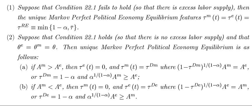
The most interesting implication of this proposition comes from the comparison of the cases with and without excess supply. When Condition 22.1 fails to hold, there is excess labor supply and taxes have no effect on wages. Anticipating this, workers favor taxes on both groups of producers to raise revenues to be redistributed to themselves. The dictatorship of the workers (“democracy”) will then generate this outcome as the political equilibrium. Clearly, this is more distortionary than either the dictatorship of the elite or the middle class, because in these political scenarios at least one of the producer groups was not taxed (but the resulting allocation is once again Pareto optimal for the same reasons as stressed above).
The situation is very different when Condition 22.1 holds. In that case, recall that both the dictatorships of the elite and of the middle class generated significant distortions owing to the factor price manipulation effect—in particular, they imposed taxes on competing producers precisely to keep wages low. In contrast, workers now dislike taxes precisely because of their effect on wages. Consequently, in this case, workers have more moderate preferences regarding taxation, and democracy generates lower taxes than both the dictatorship of the elite and the dictatorship of the middle class. This proposition therefore again highlights that which set of political institutions will generate a greater level of income per capita (or higher economic growth) depends on investment opportunities and market structure. When workers (or a subgroup that is influential in democracy) can tax entrepreneurs without suffering the consequences, democracy will generate high levels of redistributive taxation and can lead to a lower income per capita than elite or middle class dominated politics. However, when workers 1033recognize the impact of taxes on their own wages, democracy will generate more moderate political outcomes.
The simple analysis in this section therefore already gives us some clues about why there are no clear-cut relationships between political regimes and economic growth. If the forces highlighted here are important, we would expect democracy to generate higher growth under certain circumstances, for example, when the equivalent of Condition 22.1 holds. In contrast, democracy will lead to worse economic performance by pursuing populist policies and imposing high taxes when the equivalent of Condition 22.1 fails to hold. Naturally, the model presented here is very simple in many ways, and Condition 22.1 or its close cousins may not be the right ones for evaluating whether democracy or other regimes are more growth-enhancing. Nevertheless, this analysis emphasizes that democratic regimes, like the dictatorships of the elite and of the middle class, will look after the interests of the groups that have political power and the resulting allocations will often involve different types of distortions. Whether these distortions are more or less severe than those generated by alternative political regimes will depend on technology, factor endowments, and the types of policies available to the political system. In light of our analysis so far this result is not surprising, but its implications are nonetheless important to emphasize. In particular, it highlights that there are no a priori theoretical reasons to expect that there should be a simple empirical relationship between democracy and growth. On balance, we may believe that the distortions created by democracy should be less than those created by dictatorships (nondemocracies), but this will be a conclusion to be reached with more detailed theoretical and empirical analysis. Moreover, in Section 23.5 I will present another set of reasons, which I find more compelling than those implied by the simple models here, for why democracies may not generate more growth than dictatorships.
23.3. Dynamic Tradeoffs
The previous section contrasted economic allocations under different political regimes (in particular, the dictatorship of the elite, the dictatorship of the middle class and democracy, which here amounts to the dictatorship of the workers). Although the underlying economic environment was a simplified version of the infinite-horizon neoclassical growth model, the tradeoffs among the regimes were static. In this section, I will study an environment, which also involves entry into entrepreneurship, social mobility and a simple form of creative destruction. Using this environment, I will contrast the implications of democracy to oligarchy for economic performance. The emphasis will be on the dynamic tradeoffs between the two regimes.
23.3.1. The Baseline Model. The model economy is similar to that analyzed in Section 22.2 and more specifically, to the Cobb-Douglas economy in subsection 22.2.4. The economy is populated by a continuum 1 of infinitely-lived agents, each with preferences given by (22.1) as in Section 22.2. In addition, for reasons that will become clear soon, I assume that each each individual dies with a small probability ε in every period, and a mass ε of new individuals are born (with the convention that after death there is zero utility and β is the discount factor inclusive of the probability of death). I will consider the limit of this economy with ε → 0.
There are two occupations in this economy, production workers and entrepreneurs. The key difference between the models in the previous chapter (and that in the previous section) and the one here is the possibility of social mobility, i.e., the fact that individuals may choose their occupations. In particular, each agent can either be employed as a worker or set up a firm to become an entrepreneur. I assume that all agents have the same productivity as workers, but their productivity in entrepreneurship differs. In particular, agent i at time t has entrepreneurial talent/skills ¾ (t) ∈ {Al,Ah} with Al < Ah. To become an entrepreneur, an agent needs to set up a firm, if he does not have an active firm already. Setting up a new firm may be costly because of entry barriers created by existing entrepreneurs.
Each agent therefore starts period t with skill level ¾ (t) ∈ {Ah,Al} and some amount of capital ki (t) invested from the previous date (recall that, as in the models we have seen so far, capital investments are made one period in advance), and another state variable denoting whether he already possesses a firm. We will denote this by ei (t) ∈ {0,1}, with ei (t) = 1 corresponding to the individual having chosen entrepreneurship at date t-1 (for date t). More importantly, if the individual is already an “incumbent” entrepreneur at t, i.e., ei (t) = 1, this may make it cheaper for him to become an entrepreneur at date t + 1, i.e., to choose ei (t + 1) = 1, because of potential entry barriers into entrepreneurship for non-incumbents. I will refer to an agent would ei (t) = 1 as a member of the “elite” at time t, both because he will avoid the entry costs and also because in oligarchy he will be a member of the political elite making the policy choices.
In summary, at each period t, each agent makes the following decisions: an occupation choice ei (t + 1) ∈ {0,1}, and in addition if ei (t + 1) = 1, i.e., if he becomes an entrepreneur, he also makes an investment decision for next period ki (t + 1) ∈ R+. In addition, those who are currently entrepreneurs, i.e., those with ei (t) = 1, decide how much labor li (t) ∈ R∣ to hire.
Agents also make the policy choices in this society. How the preferences of various agents map into policies differs depending on the political regime, which will be discussed below. There are three policy choices. Two of those are similar to the policies we have seen so far; a tax rate τ (t) ∈ [0, T] on output and a lump-sum transfer distributed to all agents denoted
by T (t) ∈ [0, ∞). Notice that I have already imposed an upper bound on taxes τ < 1. This upper bound can be derived from the ability of individuals to hide their output in the informal sector or because of the standard distortionary effects of taxation. It simplifies the analysis to take it as given here. This parameter will have important implications on what type of political regime will lead to greater income per capita. The new policy instrument is a cost B (t) ∈ [0, ∞) imposed on new entrepreneurs setting up a firm. I assume that the entry barrier B (t) is pure waste, for example corresponding to the bureaucratic procedures that individuals have to go through to open a new business. This implies that lump-sum transfers are financed only from taxes.
An entrepreneur with skill level α⅛ (t) and capital level ki (t) produces
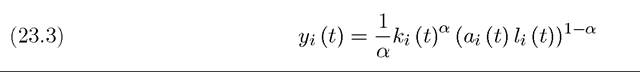
units of the final good, when he hires li (t) ∈ K ∣ units of labor. Notice that entrepreneurial skill enters the production function as a labor-augmenting productivity term. As in subsection 22.2.4, I assume that there is full depreciation of capital at the end of the period, so ki (t) is also the level of investment of entrepreneur i at time t — 1, which is in terms of the unique final good of the economy.
I will further simplify the analysis by assuming that all firms have to operate at the same size, L, so li (t) = L (see Exercise 23.6 for the implications of relaxing this assumption). Finally, I adopt the convention that the entrepreneur himself can work in his firm as one of the workers, which implies that the opportunity cost of becoming an entrepreneur is 0.
The most important assumption here is that each entrepreneur has to run the firm himself, so it is his productivity, ai (t), that matters for output. An alternative would be to allow costly delegation of managerial positions to other, more productive agents. In this case, low- productivity entrepreneurs may prefer to hire more productive managers. If delegation to managers can be done costlessly, entry barriers would create no distortions. Throughout I assume that delegation is prohibitively costly.
To simplify the expressions below, I define which corresponds to
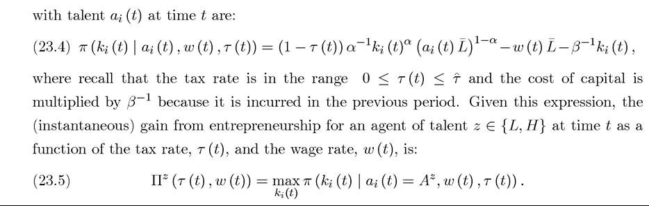
discounted per worker entry cost (and will be the relevant ob ject when we look at the profitability of different occupational choices and thus simplify the expressions). Profits (the returns to entrepreneuri gross of the cost of entry barriers) at time t are then equal to  which takes into account that investment ki (t) has to be made in the previous period, thus the opportunity cost of investment (which is forgone consumption) is multiplied by the inverse of the discount factor. This expression for profits takes into account that the entrepreneur produces an output of yi (t), pays a fraction τ (t) of this in taxes, and also pays a total wage bill of w (t) li (t). Given a tax rate τ (t) and a wage rate w (t) ≥ 0 and using the fact that li (t) = L, the net profits of an entrepreneur 1036
Note that this is the net gain to entrepreneurship since the agent receives the wage rate w (t) irrespective (either working for another entrepreneur when he is a worker, or working for himself—thus having to hire one less worker—when he is an entrepreneur). More importantly,  additional cost imposed by the entry barriers, which, like the costs of investment, is incurred in the previous period and is thus multiplied by β-1.
Labor market clearing requires the total demand for labor not to exceed the supply. Since
entrepreneurs also work as production workers, the supply is equal to 1, so:

where is the set of entrepreneurs at time t.
Finally, I specify the law of motion of entrepreneurial talent, ¾ (t), I assume that there is imperfect correlation between the entrepreneurial skill over time with the following Markov
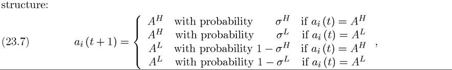
where Here σl1 is the probability that an agent has high skill in entrepre
neurship conditional on being high skill in the previous period, and σ,' is the probability transitioning from low skill to high skill. It is natural to suppose that so that
skills are persistent and low skill is not an absorbing state. What is essential for the results is imperfect correlation of entrepreneurial talent over time, i.e. so that the identities of the entrepreneurs necessary to achieve productive efficiency change over time and thus
necessitate a type of creative destruction.
The imperfect over-time correlation in ai (t) can be interpreted in three alternative and complementary ways. First, we can suppose that the productivity of an individual is not
constant over time, and changes in comparative advantage necessitate changes in the identity
1037
of entrepreneurs. Second, we can think of the infinitely-lived agents as representing dynasties, and the imperfect over-time correlation in α⅛ (t) may represent imperfect correlation between the skills of parents and children. Thrid and perhaps most interestingly, it may be that each individual has a fixed competence across different activities, and comparative advantage in entrepreneurship changes as the importance of different activities evolves over time. For example, some individuals may be better in industrial entrepreneurship, while some are better in agriculture, and as industrial activities become more profitable than agriculture, individuals who have a comparative advantage in industry should enter into entrepreneurship and those who have a comparative advantage of agriculture should exit. Both of these stories are parsimoniously captured by the Markov chain for talent given in (23.7).
This Markov chain also implies that the fraction of agents with high skill in the stationary distribution is (see Exercise 23.7):
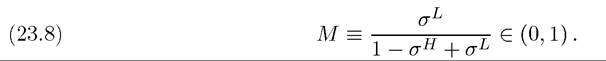
Since there is a large number (continuum) of agents, the fraction of agents with high skill at any point is M. Throughout I assume that

so that, without entry barriers, high-skill entrepreneurs generate more than sufficient demand to employ the entire labor supply. Moreover, I think of M as small and L as large; in particular, I assume L > 2, which ensures that the workers are always in the majority and simplifies the political economy discussion below.
The timing of events within every period can be summarized as follows. At the beginning of time t, ai (t), ei (t) and ki (t) are given for all individuals as a result of their decision from date t — 1. Then the following sequence of moves takes place.
(1) Entrepreneurs demand labor and the labor market clearing wage rate, w (t), is determined.
(2) The tax rate on entrepreneurs, is set.
(3) The skill level of each agent for next period, ai (t + 1),is realized.
(4) The entry barrier for new entrepreneurs b (t + 1) is set.
(5) All agents make occupational choices, ei (t + 1), and entrepreneurs make investment decisions, ki (t + 1) for next period.
Entry barriers and taxes will be set by different agents in different political regimes as will be specified below. Notice that taxes are set after the investment decisions. This raises the holdup problems discussed in the previous chapter and acts as an additional source of inefficiency. The fact that puts a limit on these holdup problems. It is also
important to note that individuals make their occupational choices and investment decisions 1038
knowing their ability level, i.e., α⅛ (t + 1) is realized before the decisions on e⅛ (t + 1) and  Notice also that if an individual does not operate his firm, he loses “the license”, so next time he wants to set up a firm, he needs to incur the entry cost (and the assumption that li (t) = L rules out the possibility of operating the firm at a much smaller scale). Finally, we need to specify the initial conditions: I assume that the distribution of talent in the society is given by the stationary distribution, nobody starts out as an entrepreneur, so that ei (-1) = 0 for all i, and the initial level of capital holdings is not important, since negative consumption is allowed, thus individuals can always increase their capital holdings by choosing a negative level of consumption.
Let us again focus on Markov Perfect Political Economy Equilibrium, where strategies are only a function of the payoff relevant states. For individual i the payoff relevant state at time t includes his own state (ei (t),ai (t),ki (t),ai (t + 1)),3 and potentially the fraction of entrepreneurs that are high skill, denoted by μ (t), and defined as

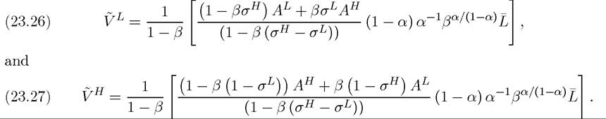
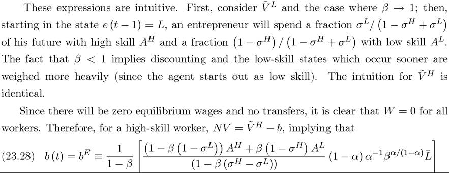
The equilibrium can be characterized by writing the net present discounted values of different agents recursively and then characterizing the optimal strategies within each time period by backward induction. I start with the “economic equilibrium,” which is the equi- 
where Πz is given by (23.10) and now crucially depends on the skill level of the agent, and  is the continuation value for an entrepreneur of type z:

An entrepreneur of ability Az also receives the wage w (t) (working for his own firm) and the transfer T (t), and in addition makes profits equal to The following period,
this entrepreneur has high skill with probability σz and low skill with probability 1 — σz, and conditional on the realization of this event, he decides whether to remain an entrepreneur or become a worker. Two points are noteworthy here. First, in (23.15), in contrast to the expression in (23.13), there is no additional cost of becoming an entrepreneur since this individual already owns a firm. Second, if an entrepreneur decides to become a worker, he obtains the value as given by the expressions in (23.13) so that the next time he wishes to operate a firm, he has to incur the cost of doing so.
Inspection of (23.13) and (23.15) immediately reveals that the occupational choices of individuals for time t will depend on the net value of entrepreneurship conditional on their current occupational status, et (t — 1) = e. We write this is

which is defined as a function of an individual’s skill a and current entrepreneurship status, e. The last term is the entry cost incurred by agents with e = 0. The max operators in (23.13) and (23.15) imply that if NV > 0 for an agent, then he prefers to become an entrepreneur.
Who will become an entrepreneur in this economy? The answer depends on the NV’s. Standard dynamic programming arguments from Chapters 6 and 16, combined with the fact 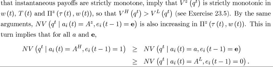 In other words, the net value of entrepreneurship is highest for high-skill existing entrepreneurs, and lowest for low-skill workers. However, it is unclear ex ante whether
 is greater, that is, whether entrepreneurship is more profitable for incumbents with low skill or for outsiders with high skill, who will have to pay the entry cost.
We can then define two different types of equilibria:
(1) Entry equilibrium where all entrepreneurs have αt (t) = Ah.
(2) Sclerotic equilibrium where agents with e⅛ (t — 1) = 1 remain entrepreneurs irrespective of their productivity.
An entry equilibrium requires the net value of entrepreneurship to be greater for a nonelite high skill agent than for a low-skill elite. Let us define wH (t) as the threshold wage
of the elite for a high-skill agent. Naturally, this benefit will depend on the sequence of
policies, for example, it will be larger when there are greater entry barriers in the future. Consequently, if wL (t) < wh (t), the total benefit of becoming an entrepreneur for a non-elite high-skill agent exceeds the cost. Equation (23.17) is explained similarly. Evidently, a wage rate lower than both wL (t) and wH (t) would lead to excess demand for labor and could not be an equilibrium. Consequently, the condition for an entry equilibrium to exist at time t
can simply be written as a comparison of the two thresholds determined above:

A sclerotic equilibrium emerges, on the other hand, when the converse of (23.18) holds. Moreover, in an entry equilibrium, i.e., when (23.18) holds, we must have that
 If it were strictly positive, or in other words, if the wage were less than w (t), all agents with high skill would strictly prefer to become entrepreneurs, which is not possible since, by assumption,
 . This argument also shows that the total number (measure) of entrepreneurs in the economy will be
 Then, from (23.10), (23.12) and (23.14), the equilibrium wage, which will be denoted wE (t), is
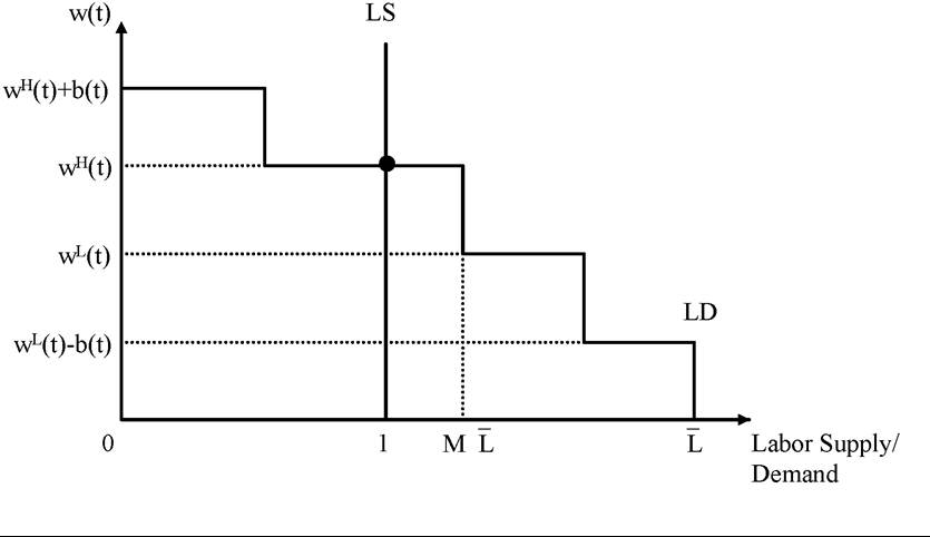
Figure 23.1. Labor market equilibrium when (23.18) holds.
equal to

Note also that when (23.18) holds, naturally so low-
skill incumbents would be worse off if they remained as entrepreneurs at the equilibrium wage rate wE (t).
Figure 23.1 illustrates the entry equilibrium diagrammatically by plotting labor demand and supply in this economy. Labor supply is constant at 1, while labor demand is decreasing as a function of the wage rate. This figure is drawn for the case where condition (23.18) holds, so that there exists an entry equilibrium. The first portion of the curve shows the willingness to pay of high-skill incumbents, i.e., those who start with et (t — 1) = 1 but have high entrepreneurial skills a,{ (t) = Ah. This marginal willingness is wH (t) + b (t) (since entrepreneurship is as profitable for them as for high-skill potential entrants and they do not have pay the entry cost). The second portion is for high-skill potential entrants—those with ei (t — 1) = 0 and ai (t) = Ah—and is equal to wH (t). These two groups together demand ML > 1 workers, ensuring that labor demand intersects labor supply at the wage given in (23.19).
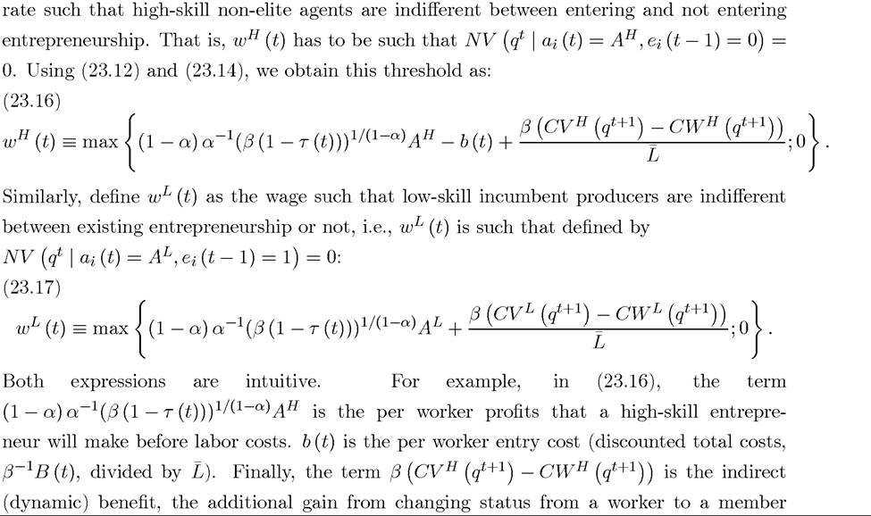
Figure 23.2. Labor market equilibrium when (23.18) does not hold.
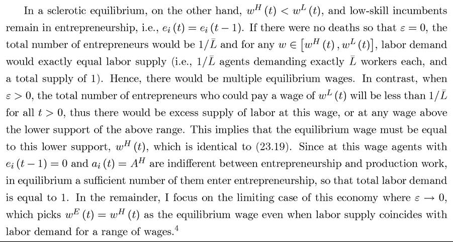
Figure 23.2 illustrates this case diagrammatically. Because (23.18) does not hold in this case, the second flat portion of the labor demand curve is for low-skill incumbents
4In other words, the wage wH (t) at ε = 0 is the only point in the equilibrium set where the equilibrium correspondence is (lower-hemi) continuous in ε (recall the definition of lower hemi-continuity in Definitions A.24 and A.25 in Appendix Chapter A). In fact, the feature that there will be multiple equilibrium wage levels in dynamic models with entry barriers is not a feature of the setup here, which involves two types of entrepreneurs. This is demonstrated in Exercise 23.13.
(ei (t — 1) = 1 and ai (t) = Al) who, given the entry barriers, have a higher marginal product of labor than high-skill potential entrants.
The equilibrium law of motion of the fraction of high-skill entrepreneurs, μ (t), is:

starting with some μ (0). The exact value of μ (0) will play an important role below. Recall that we have assumed above that et ( — 1) = 0 for all i. Under this assumption, any b (0) would apply equally to all potential entrants and as long as it is not so high as to shut down the economy, the equilibrium would involve μ (0) = 1. I consider μ (0) = 1 to be the baseline case in the analysis below. While an economy with et (—1) = 0 is a plausible benchmark, I will also discuss below how the results differ if et ( — 1) = 1 for some i, so that the economy already starts with some privileged “elites” at the initial period. This will also open the way for a discussion of the potential adverse consequences of other selection mechanisms into entrepreneurship in the initial period.
To obtain a full political equilibrium, we need to determine the policy sequence pt. I consider two extreme cases: (1) Democracy: the policies b (t) and τ (t) are determined by majoritarian voting, with each agent having one vote. (2) Elite control (Oligarchy): the policies b (t) and τ (t) are determined by majoritarian voting among the elite—the current entrepreneurs—at time t.
23.3.2. Democracy. A democratic equilibrium is a MPE where b (t) and τ (t) are determined by majoritarian voting at time t. The timing of events implies that the tax rate at time t, τ (t), is decided after investment decisions, whereas the entry barriers are decided before. The assumption L > 2 above ensures that workers (non-elite agents) are always in the ma jority.
At the time taxes are set, investments are sunk, agents have already made their occupation choices, and workers are in the majority. Therefore, taxes will be chosen to maximize per capita transfers given by
which takes into account that k (t) is already given from the investment in the previous period. Since this expression is increasing in the optimal tax for a worker
is In view of this, total tax revenues are

The entry barrier, b (t), is then set at the end of period t — 1 (before occupational choices) to maximize this expression. Low-productivity workers (with
know that they will remain workers, and in MPE, the policy choice at time t has no influence 1045
Inspection of (23.19) and (23.21) immediately shows that wages and tax revenue are both maximized when b (t + 1) = 0 for all t, so the democratic equilibrium will not impose any entry barriers. This is intuitive; workers have nothing to gain by protecting incumbents, and a lot to lose, since such protection reduces labor demand and wages. Since there are no entry barriers, only high-skill agents will become entrepreneurs, or in other words ei (t) = 1 only if Oi (t) = Ah at all t. Given this stationary sequence of MPE policies, we can use the value functions (23.12) and (23.14) to obtain

An important feature of the democratic equilibrium is that aggregate output is constant over time. This will contrast with the oligarchic equilibrium, where the skill composition of entrepreneurs and the level of output will change over time. Another noteworthy feature is that there is perfect equality because the excess supply of high-skill entrepreneurs ensures that they receive no rents.
It is useful to note that YD corresponds to the level of output inclusive of consumption and investment. “Net output” and consumption can be obtained by sub net output. I focus on output only because the expressions are slightly simpler.
23.3.3. Oligarchic Equilibrium. In oligarchy, policies are determined by majoritarian
Let us start with the taxation decision among those with e⅛ (t) = 1 and also impose the following condition:
Condition 23.1.
When this condition is satisfied, both high-skill and low-skill entrepreneurs prefer zero taxes, i.e., τ (t) = 0. I simplify the analysis here by assuming that this condition holds. Exercise 23.10 discusses the case when this condition is relaxed. Intuitively, Condition 23.1 requires the productivity gap between low and high-skill elites not to be so large that low-skill elites wish to tax profits in order to indirectly transfer resources from high-skill entrepreneurs to themselves.
When Condition 23.1 holds, the oligarchy will always choose τ (t) = 0. Then, at the stage of deciding the entry barriers, high-skill entrepreneurs would like to choose b (t) to maximize Vh, and low-skill entrepreneurs would like to maximize Vl (both groups anticipating that τ (t) = 0). Both of these expressions are maximized by setting a level of the entry barrier that ensures the minimum level of equilibrium wages. Recall from (23.19) that equilibrium wages in this case are still given by wE (t) = wH (t), so they will be minimized by ensuring that w (t) = 0, i.e., by choosing any

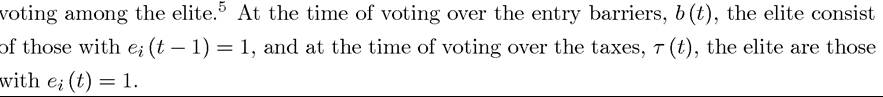
5Notice that this assumption means political power rests with current entrepreneurs. As discussed in the previous chapter, there may often be a decoupling between economic and political power, so that key decisions are not made by current entrepreneurs, but by those who are politically powerful for historical or other reasons. The analysis in the previous chapter and also in Section 23.2 in this chapter illustrated the distortionary policies that would arise from such decoupling. The model here goes to the other extreme and places all political power in the hands of the current entrepreneurs and highlights a different set of inefficiencies that this will cause.
Without loss of any generality, let us assume that they will set the entry barrier as b (t) = bE (t) in this case.
An oligarchic equilibrium then can be defined as a policy sequence wage sequence
  and economic decisions
 such that
 and
and constitute an economic equilibrium given
  , and
, and is such
 In the oligarchic
equilibrium, there is no redistributive taxation and entry barriers are sufficiently high to ensure a sclerotic equilibrium with zero wages.
Imposing we can solve for the equilibrium values of high-
and low-skill entrepreneurs from the value functions (23.14) as
is sufficient to ensure zero equilibrium wages.
In this oligarchic equilibrium, aggregate output is:
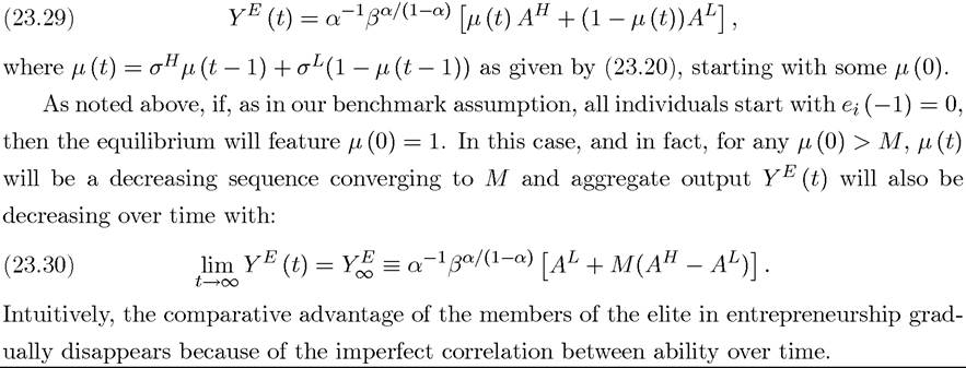
Nevertheless, it is also possible to imagine societies in which μ (0) < M, because there is some other process of selection into the oligarchy in the initial period that is negatively correlated with skills in entrepreneurship. In this case, somewhat paradoxically, μ (t) and thus Ye (t) would be increasing over time. While interesting in theory, this case appears less relevant in practice, where we would expect at least some positive selection in the initial period, so that high-skill agents are more likely to become entrepreneurs at time t = 0 and μ (0) > M.
Another important feature of the oligarchic equilibrium is that there is a high degree of (income) inequality. Wages are equal to 0, while entrepreneurs earn positive profits—in fact, each entrepreneur earns yi (t) L (gross of investment expenses), where yi (t) depends on the current skill level of the entrepreneur. Since wages are equal to 0, total entrepreneurial earnings are equal to aggregate output. This contrasts with relative equality in democracy.
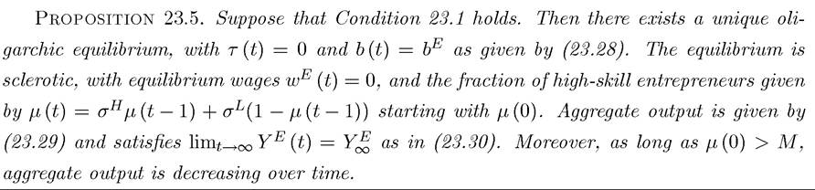
Proof. See Exercise 23.8. ?
23.3.4. Comparison Between Democracy and Oligarchy. The first important result in the comparison between democracy and oligarchy is that if initial selection into entrepreneurship is on the basis of entrepreneurial skills (e.g., because so that
μ (0) = 1, then aggregate output in the initial period of the oligarchic equilibrium, Ye (0), is greater than the constant level of output in the democratic equilibrium, YD. In other words,

Therefore, oligarchy initially generates greater output than democracy, because it is protecting the property rights of entrepreneurs (whereas democracy is imposing distortionary taxes on entrepreneurs). However, the analysis also shows that, in this case, Ye (t) declines over time, while Yd is constant. Consequently, the oligarchic economy may subsequently fall r
,
1049
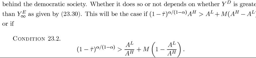
If Condition 23.2 holds, then at some point the democratic society will overtake (“leapfrog") the oligarchic society.
As noted above, it is possible to imagine societies in which even in the initial period, there are “elites” that are not selected into entrepreneurship on the basis of their skills. In this case, we will typically have μ (0) < 1. In the extreme case where there is negative selection into entrepreneurship in the initial period, we have μ (0) < M. To analyze these cases, let us define

It can be verified that as long as μ (0) > μ (0), oligarchy will generate greater output than democracy in the initial period. Notice also that μ (0) > M if and only if Condition 23.2 holds.
This discussion and inspection of Condition 23.2 establish the following result (proof in the text):
Proof. See Exercise 23.9. ?
This proposition implies that when μ (0) is not excessively low (i.e., when there is no negative correlation between initial entry into entrepreneurship and skills), an oligarchic society will start out as more productive than a democratic society, but will decline over time.
This proposition shows that oligarchy is more likely to be relatively inefficient in the long run:
(1) when T is low, meaning that democracy is unable to pursue highly populist policies with a high degree of redistribution away from entrepreneurs/capitalists. The
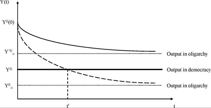
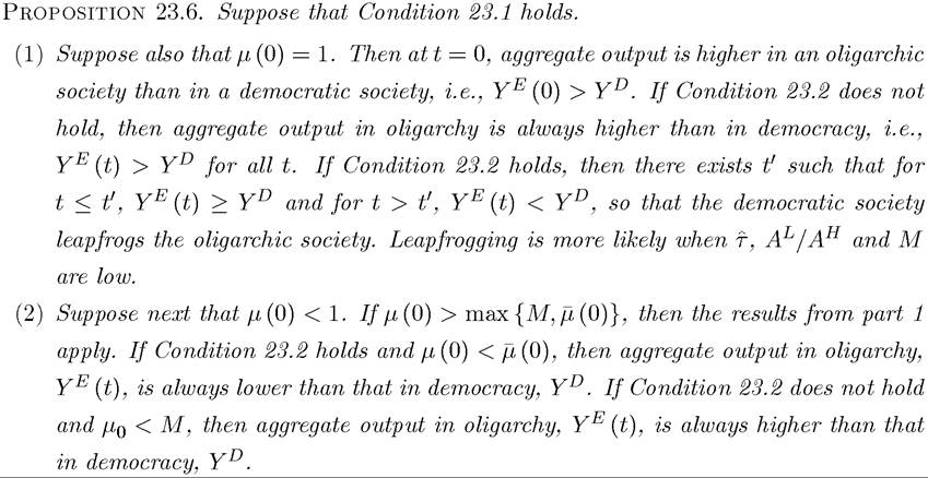
FIGURE 23.3. Dynamic comparison of output in oligarchy and democracy. The dashed line represents output in oligarchy when Condition 23.2 holds, and the solid line represents output in oligarchy when this condition does not hold.
parameter may correspond both to certain institutional impediments limiting redistribution, or more interestingly, to the specificity of assets in the economy; with greater specificity, taxes will be limited, and redistributive distortions may be less important.
(2) when Ah is high relative to Al, so that the creative destruction process—the selection of high-skill agents for entrepreneurship—is important for the efficient allocation of resources.
(3) M is low, so that a random selection of agents contains a small fraction of high- skill agents, making oligarchic sclerosis highly distortionary. Alternatively, M is low when uh is low, so oligarchies are more likely to lead to low output in the long run when the efficient allocation of resources requires a high degree of “churning” in the ranks of entrepreneurs, which is another measure of the importance of creative destruction.
On the other hand, if the extent of taxation in democracy is high and the failure to allocate the right agents to entrepreneurship only has limited costs, then an oligarchic society will generate greater output than a democracy in the long run.
These comparative static results may be useful in interpreting why, as discussed in Section
23.1, the Northeastern United States so conclusively outperformed the Caribbean plantation 1051
economies during the 19th century. First, the American democracy was not highly redistributive, corresponding to low τ in terms of the model here. More important, the 19th century was the age of industry and commerce, where the allocation of high-skill agents to entrepreneurship appears to have been probably quite important, and potentially only a small fraction of the population were really talented as inventors and entrepreneurs. This can be thought of as a low value of Al/Ah and M.
Figure 23.3 illustrates the case with and depicts
both the situation in which Condition 23.2 holds and the converse. The thick flat line shows the level of aggregate output in democracy, YD. The other two curves depict the level of output in oligarchy, Ye (t), as a function of time for the case where Condition 23.2 holds and for the case where it does not. Both of these curves asymptote to some limit, either or
or  which may lie below or above YD. The dashed curve shows the case where Condition 23.2 holds, so after date t', oligarchy generates less aggregate output than democracy. When Condition 23.2 does not hold, the solid curve applies, and aggregate output in oligarchy asymptotes to a level higher than YD.
Naturally, both of these major results, the greater short-term efficiency and the dynamic costs of oligarchy, are derived from the underlying assumptions of the model. In addition to μ (0) being sufficiently large, the first result is a consequence of the assumption that the only source of distortion in oligarchy is the entry barriers. In practice, an oligarchic society could pursue other distortionary policies to reduce wages and increase profits, in which case it might generate lower output than a democratic society even at time t = 0. I will emphasize how these costs arise and affect equilibrium dynamics in Section 23.5 below. The dynamic costs of oligarchy are also stark in this model, since output and distortions in democracy are constant, whereas the allocation of talent deteriorates in oligarchy because of the entry barriers. In more general models, democracy may also create intertemporal distortions. For example, if democracy is expected to tax capital incomes in the future and and there is less than full depreciation, this will create dynamic distortions by affecting the whole sequence of investment levels, though in this case, it is also reasonable to think that oligarchy may tax human capital more, creating similar distortions. Which set of distortions dominate is an empirical question. Nevertheless, the dynamic distortions of oligarchy emphasized in this paper are new and potentially important, and thus need to be considered in evaluating the allocative costs of these regimes.
The second part of the proposition also highlights the role of selection of individuals into entrepreneurship (and oligarchy) in the initial period. It shows that the results highlighted so far hold even if μ (0) is less than one, as long as it is not very small. On the other hand, if μ (0) is very small to start with, oligarchy may always generate less output than democracy, and in fact, if μ (0) starts out less than M, oligarchy may even have increasing level of
output. A very low level of μ (0) may emerge if the oligarchy is founded by individuals that are talented in non-economic activities (e.g., by elites specialized in fighting in pre-modern times) and these non-economic talents are negatively correlated with entrepreneurial skills. Nevertheless, as noted above, a significant amount of positive selection on the basis of skills even in the initial period seems to be the more reasonable case.
On the basis of this analysis, the current model not only adds to the arguments we have made already, that there is no unambiguous theoretical result on whether democracy or nondemocracy will generate greater growth, but it also highlights a different dimension of the tradeoff between different regimes—that related to the dynamics they imply. While democracy may create short-run distortions, it can lead to better long-run performance because it avoids political sclerosis—that is, incumbents becoming politically powerful and erecting entry barriers against new and better entrepreneurs. This model therefore suggests precisely the type of patterns we already discussed in Section 23.1; lack of a clear relationship between democracy and growth over the past 50 years combined with the examples of democracies that have been able to achieve industrialization during critical periods in the 19th century. In fact, a simple extension of the framework here provides additional insights that are useful in thinking about why democracies may be successful in preventing political sclerosis; the forces highlighted here also suggest that democracies are more “flexible” than oligarchies. In particular, Exercise 23.12 considers a simple extension of the framework here and demonstrates that democracies will typically be better able to adapt to the arrival of new technologies, because there are no incumbents with rents to protect, who can successfully block or slow down the introduction of new technology. This type of flexibility might, ultimately, be one of the more important advantages of democratic regimes.
Even though the model presented in this section provides a range of ideas and comparative static results that are useful for understanding the comparative development experiences of democratic and nondemocratic regimes, like the model discussed in the previous section, it focuses on the costs of democracy resulting from its more redistributive nature—in particular, it emphasizes that democratic regimes redistribute income away from the rich and the entrepreneurs towards the poorer segments of the society and this leads to distortions reducing income per capita. An alternative source of distortions in democracy, which will complement the mechanisms discussed here, will be the resistance of the elite against democratic redistributive policies, which will often lead to additional inefficiencies. This will be discussed in Section 23.5.
Before doing this, however, it is useful to return to the induced preferences over different regimes. As a first step in this direction, let us look at income inequality and the preferences of different groups over regimes. First, it is straightforward to see that oligarchy always generates more (consumption) inequality relative to democracy, since the latter has perfect equality—the net incomes and consumption of all agents are equalized in democracy because of the excess supply of high-skill entrepreneurs.
Moreover, non-elites are always better off in democracy than in oligarchy, where they receive zero income. In contrast, and more interestingly, it is possible for low-skill elites to be better off in democracy than in oligarchy (though high-skill elites are always better off in oligarchy). This point will play a role in our first result on regime change in subsection
23.3.5, so it is useful to understand the intuition. Recall that the utility of low-skill elites in oligarchy is given by (23.26) above, whereas combining (23.22), (23.23) and (23.24), these low-skill agents in democracy would receive:
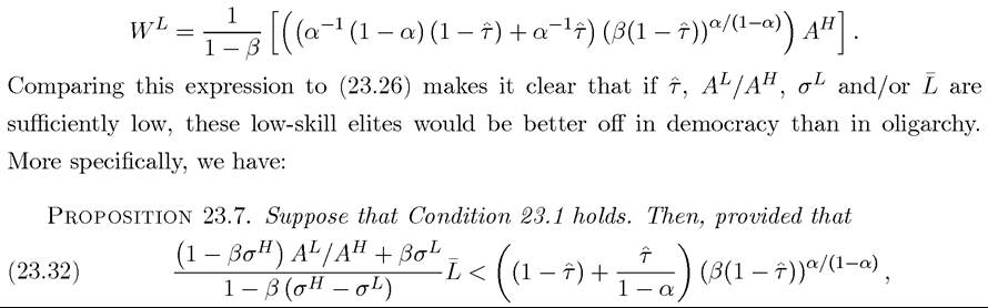
low-skill elites would be better off in democracy.
Proof. See Exercise 23.11 ?
Note, however, that so far even when (23.32) holds, low-skill elites prefer to remain in entrepreneurship. This is because, given the structure of the political game, if the low-skill incumbent elites give up entrepreneurship, the new entrepreneurs will make the political choices, and they will naturally choose high entry barriers and no redistribution. Therefore, by quitting entrepreneurship, low-skill elites would be giving up their political power. Consequently, they are choosing between being elites and being workers in oligarchy, and clearly, the former is preferred.
23.3.5. First Thoughts on Regime Changes. I have so far characterized the political equilibrium under two different scenarios; democracy and oligarchy. Which political system prevails in a given society was treated as exogenous. Why are certain societies democratic, while others are oligarchic? One possibility is to appeal to historical accident, while another is to construct a “behind-the-veil” argument, whereby whichever political system leads to greater efficiency or ex ante utility would prevail. This approach is not satisfactory, however. Political regimes matter precisely because they regulate the conflict of interest between different groups (in this context, between workers and entrepreneurs). The behind-the-veil approach is unsatisfactory, since it recognizes and models this conflict to determine the equilibrium within a particular regime, but then ignores it when there is a choice of regime.
Moreover, this approach does not provide a framework for the analysis of regime changes in the context of a dynamic equilibrium.
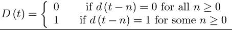
A more satisfactory approach would be to use the induced preferences of the agents over political regimes and analyze a game over the determination of political institutions, where agents have these induced preferences. Broadly speaking two types of processes can lead to political change in this case. The first is some type of voluntary agreement within the society (or within a decisive subset of the society) involving an equilibrium change in political institutions. The second results from conflict over political institutions. In this subsection, I will start with the first alternative, which is simpler and fits well with the model presented here. However, most political changes in practice are better approximated by the second approach, and this will be the topic of the next two sections. For now, let us return to our basic model in this section and assume that μ (0) = 1. Let us also make one modification to the baseline framework: the current elite can now vote to disband oligarchy, upon which a permanent democracy is established (previously, for example, in Proposition 23.7, such a vote was not allowed). I denote this choice by d (t) ∈ {0,1}, with 0 standing for continuation with the oligarchic regime. To describe the law of motion of the political regime, let us denote oligarchy by D (t) = 0 and democracy by D (t) = 1. Since transition to democracy is permanent, we have
Voting over d (t) in oligarchy is at the same time as voting over b (t) (there are no votes over d (t) in democracy, since a transition to democracy is permanent), so agents with get to vote over these choices. I assume that after the vote for d (t) = 1, there is immediate democratization and all agents participate in the vote over taxes starting in period t.
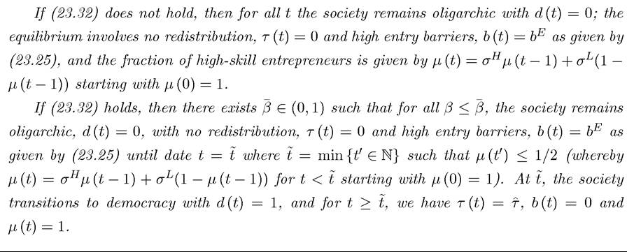
First, imagine a situation where condition (23.32) does not hold so that even low-skill elites are better off in oligarchy. Then all elites will always vote for d (t) = 0, and also choose b (t) = bE and τ (t) = 0 (as in Proposition 23.5). Hence, in this case, the equilibrium remains oligarchic throughout.
What happens when (23.32) holds? Current low-skill elites, i.e., those with e⅛ (t) = 1 and would be better off in democracy (recall Proposition 23.7). If they vote
for d (t) = 0, they stay in oligarchy, which gives them a lower payoff. If, instead, they vote for d (t) = 1 and b (t) = 0, then this will lead to democracy. Consequently, following this vote, high-skill agents enter entrepreneurship and there are redistributive taxes at the rate  as in Proposition 23.4. Now, when they are in the majority, low-skill elites can induce a transition to a permanent democracy by voting for d (t) = 1. Since μ (0) = 1, however, they are initially in the minority, and the oligarchic equilibrium persists for a while. Nevertheless, the fraction of high-skill elites will decrease over time. Provided that M < 1/2 and that
entry barriers are kept throughout, low-skill agents will eventually become the majority and succeed in disbanding the oligarchic regime. One complication is that as μ (t) approaches 1/2, high-skill elites may prefer to temporarily reduce the entry barrier and include new entrepreneurs in order to prevent the disbanding of the regime. Nevertheless, this strategy will not be attractive when the future is discounted heavily. Consequently, we can establish the following proposition:
Proposition 23.8. Suppose that Condition 23.1 holds, M < 1/2 and the society starts as oligarchic.
Proof. See Exercise 23.14. ?
Intuitively, when (23.32) holds, low-skill entrepreneurs are better off transitioning to democracy than remaining in the oligarchic society, while high-skill entrepreneurs are always better off in oligarchy. Because they discount the future heavily, high-skill entrepreneurs are not willing to reduce entry barriers and sacrifice current profits. As a result, the society remains oligarchic as long as high-skill entrepreneurs are in the majority, i.e., as long as and the first period in which low-skill entrepreneurs become majority within the oligarchy, i.e., at
 such that μ (t) < 1/2 for the first time, the oligarchy disbands itself transitioning to a democratic regime (and at that point μ (t) jumps up to 1).
This configuration is especially interesting when Condition 23.2 holds such that oligarchy ultimately would have led to lower output than democracy. In this case, as long as (23.32) holds, oligarchy transitions to democracy avoiding the long-run adverse efficiency consequences of oligarchy (though when this condition does not hold, oligarchy survives forever with negative consequences for efficiency and output). This extension therefore provides a simple framework for thinking about how a society can transition from oligarchy to a more democratic system, before the oligarchic regime becomes excessively costly. Interestingly, 1056
however, the reason for the transition from oligarchy to democracy is not increased inefficiency in the oligarchy, but conflict between high and low-skill agents within the oligarchy; the transition takes place when the low-skill elites become the majority.
The result presented in Proposition 23.8 only leads to equilibrium regime change when (23.32) holds. When it fails to hold, this proposition states that society will remain permanently as an oligarchy (provided that it starts as an oligarchy). However, the induced preferences of different agents are radically opposed to each other. Those who are the incumbent entrepreneurs—the elite—are happy in oligarchy, whereas those left out of the elite have the worst possible allocation, with zero wages and zero consumption. They are also the majority. Can we expect the oligarchic system that serves the interests of a small minority of the population to last forever? To answer this question, we need to introduce additional ideas about how political change can happen when there is social conflict over the set of political institutions in the society. This is what I turn to next.
23.4.