Preliminaries

To prepare for this analysis, let us consider an economy consisting of a unit measure of infinitely-lived households. By a unit measure of households I mean an uncountable number of households, for example, the set of households H could be represented by the unit interval [0,1].

Households in this economy may be truly “infinitely lived,” or alternatively they may consist of overlapping generations with full (or partial) altruism linking generations within the household. Throughout, I equate households with individuals, and thus ignore all possible sources of conflict or different preferences within the household. In other words, I assume that households have well-defined preference orderings.

As in basic general equilibrium theory, let us suppose that preference orderings can be represented by utility functions. In particular, suppose that each household h has an instan­taneous utility function given by

where Uh : R∣∣→ R is increasing and concave and ¾ (t) is the consumption of household h. I take the domain of the utility function to be R ∣ rather than R, so that negative levels of consumption are not allowed.

The instantaneous utility function captures the utility that an individual (or household) derives from consumption at time t. It is therefore not the same as a utility function specifying a complete preference ordering over all commodities—here consumption levels in all dates. For this reason, the instantaneous utility function is sometimes also referred to as the “felicity function”.

There are two major assumptions in writing an instantaneous utility function. First, it imposes that the household does not derive any utility from the consumption of other households, so consumption externalities are ruled out. Second, in writing the instantaneous utility function, I already imposed that overall utility is time-separable, that is, instantaneous utility at time t is independent of the consumption levels at past or future dates. This second feature is important in enabling us to develop tractable models of dynamic optimization.

Finally, let us introduce a third assumption and suppose that households discount the future “exponentially”—or “proportionally”. In discrete time, and ignoring uncertainty, this implies that household preferences at time t = 0 can be represented as where β_h ∈ (0,1) is the discount factor of household h. This functional form implies that the weight given to tomorrow’s utility is a fraction β_h of today’s utility, and the weight given to the utility the day after tomorrow is a fraction βh of today’s utility, and so on. Exponential discounting and time separability are convenient for us because they naturally ensure “time-consistent” behavior.

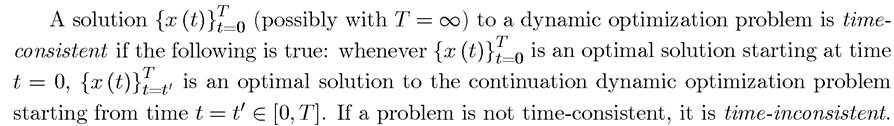
Time-consistent problems are much more straightforward to work with and satisfy all of the standard axioms of rational decision-making.

There is a natural analog to (5.1) in continuous time, again incorporating exponential discounting, which is introduced and discussed below (see Chapter 7).

The expression in (5.1) ignores uncertainty in the sense that it assumes the sequence of consumption levels for householdis known with certainty. If instead this

sequence were uncertain, we would need to look at expected utility maximization. Most growth models do not necessitate an analysis of behavior under uncertainty, but a stochastic version of the neoclassical growth model is the workhorse of much of the rest of modern macroeconomics and will be presented in Chapter 17. For now, it suffices to say that in the presence of uncertainty, u⅛ (∙) should be interpreted as a “Bernoulli utility function,” defined over risky acts, so that the preferences of household h at time t = 0 can be represented by the following von Neumann-Morgenstern expected utility function:

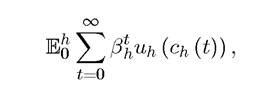
whereis the expectation operator with respect to the information set available to house­hold h at time t = 0.

The formulation so far indexes individual utility function, u⅛ (∙), and the discount factor, β_h, by “h” to emphasize that these preference parameters are potentially different across households. Households could also differ according to their income processes. For example, each household could have effective labor endowments ofthus a sequence of labor

income ofwhere w (t) is the equilibrium wage rate per unit of effective labor.

Unfortunately, at this level of generality, this problem is not tractable. Even though we can establish some existence of equilibrium results, it would be impossible to go beyond that. Proving the existence of equilibrium in this class of models is of some interest, but our focus is on developing workable models of economic growth that generate insights about the process of growth over time and cross-country income differences. I will therefore follow the standard approach in macroeconomics and assume the existence of a representative household.

5.2.