The Representative Household

When we say that an economy admits a representative household, this means that the preference (demand) side of the economy can be represented as if there were a single house­hold making the aggregate consumption and saving decisions (and also the labor supply decisions when these are endogenized) subject to an aggregate budget constraint.

welfare comparisons, but is valid under much more stringent conditions. I return to a further discussion of these issues below.

Let us start with the simplest case that will lead to the existence of a representative household. Suppose that each household is identical, that is, each has the same discount factor β, the same sequence of effective labor endowmentsand the same instantaneous

utility function

whereis increasing and concave and ¾ (t) is the consumption of household

h. Therefore, there is really a representative household in this case. Consequently, again ignoring uncertainty, the preference side of the economy can be represented as the solution to the following maximization problem starting at time t = 0:

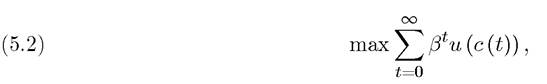
where β ∈ (0,1) is the common discount factor of all the households, and c (t) is the con­sumption level of the representative household.

The economy described so far admits a representative household rather trivially; all house­holds are identical. In this case, the representative household’s preferences, (5.2), can be used not only for positive analysis (for example, to determine what the level of savings will be), but also for normative analysis, such as evaluating the optimality of equilibria.^[VII]

Often, we may not want to assume that the economy is indeed inhabited by a set of identical households, but instead assume that the behavior of the households can be modeled as if it were generated by the optimization decision of a representative household. Naturally, this would be more realistic than assuming that all households are identical. Nevertheless, this is not without any costs. First, in this case, the representative household will have positive meaning, but not always a normative meaning (see below). Second, it is not in fact true that most models with heterogeneity lead to a behavior that can be represented as if it were generated by a representative household.

In fact most models do not admit a representative household. To illustrate this, let us consider a simple exchange economy with a finite number of commodities and state an important theorem from general equilibrium theory. In preparation for this theorem, recall that in an exchange economy, we can think of the object of interest as the excess demand functions (or correspondences) for different commodities. Let these be denoted by x (p) when the vector of prices is p. The demand side of an economy will admit a representative household if these excess demands, x (p), can be modeled as if they result from the maximization problem of a single consumer.

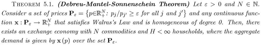
Proof. See Debreu (1974) or Mas-Colell, Winston and Green (1995), Proposition 17.E.3.

?

Therefore, the fact that excess demands result from aggregating the optimizing behavior of households places few restrictions on the form of these demands.

Nevertheless, this result is partly an outcome of very strong income effects. Special but approximately realistic preference functions, as well as restrictions on the distribution of in­come across individuals, enable us to rule out arbitrary aggregate excess demand functions. To show that the representative household assumption is not as hopeless as Theorem 5.1 sug­gests, I now present a special and relevant case in which aggregation of individual preferences is possible and enables the modeling of the economy as if the demand side was generated by a representative household.

To prepare for this theorem, consider an economy with a finite number N of commodities and recall that an indirect utility function for household h, v∣_i (p, y^h), specifies the household’s (ordinal) utility as a function of the price vector p = (pι,...,pκ) and the household’s income y^h. Naturally, any indirect utility function v⅛ (p,y^h) has to be homogeneous of degree 0 in p and y.

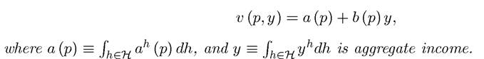
Theorem 5.2. (Gorman's Aggregation Theorem) Consider an economy with a finite number N < ∞ of commodities and a set H of households. Suppose that the preferences of household h ∈ H can be represented by an indirect utility function of the form

then these preferences can be aggregated and represented by those of a representative house­hold, with indirect utility

Proof.

This theorem implies that when preferences admit this special quasi-linear form, aggre­gate behavior can indeed be represented as if it resulted from the maximization of a single household. This class of preferences are referred to as Gorman preferences after Terrence Gorman, who was among the first economists studying issues of aggregation and proposed the special class of preferences used in Theorem 5.2. The quasi-linear structure of these pref­erences limits the extent of income effects and enables the aggregation of individual behavior. Notice that instead of the summation, this theorem used the integral over the set H to allow for the possibility that the set of households may be a continuum. The integral should be thought of as the “Lebesgue integral,” so that when H is a finite or countable set, is indeed equivalent to the summationNote also that this theorem is stated for

an economy with a finite number of commodities. This is only for simplicity, and the same result can be generalized to an economy with an infinite or even a continuum of commodities. However, for most of this chapter, I restrict attention to economies with either a finite or a countable number of commodities to simplify notation and avoid technical details.

Note also that for preferences to be represented by an indirect utility function of the Gorman form does not necessarily mean that this utility function will give exactly the indirect utility in (5.3). Since, in the absence of uncertainty, a monotonic transformation of the utility function has no effect on behavior (but affects the indirect utility function), all that is required in models without uncertainty is that there exists a monotonic transformation of the indirect utility function that takes the form given in (5.3).

Another attractive feature of Gorman preferences for our purposes is that they contain some commonly-used preferences in macroeconomics. To illustrate this, let us start with the following example:

EXAMPLE 5.1. (Constant Elasticity of Substitution Preferences) A very common class of preferences used in industrial organization and macroeconomics are the constant elasticity of substitution (CES) preferences, also referred to as Dixit-Stiglitz preferences after the two economists who first used these preferences. Suppose that each household denoted by h ∈ H has total income y^h and preferences defined over j = 1,...,N goods given by

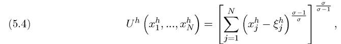
where σ ∈ (0, ∞) and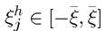is a household specific term, which parameterizes whether

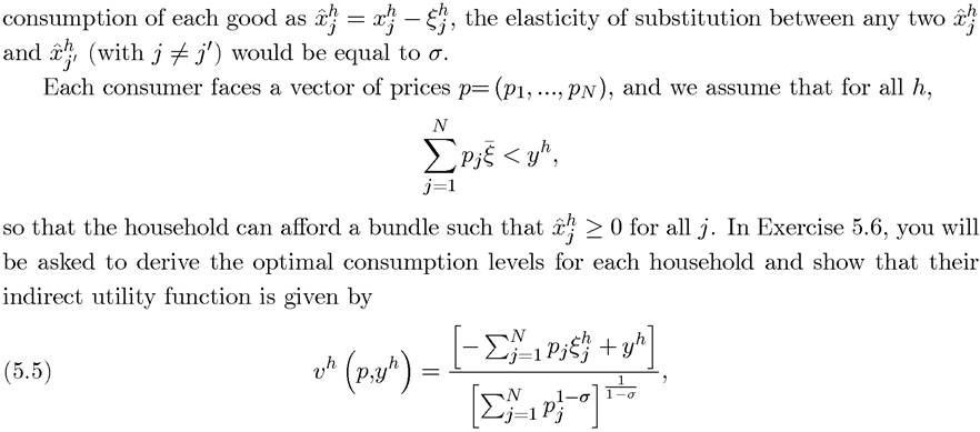
the particular good is a necessity for the household. For example,may mean that household h needs to consume at least a certain amount of good j to survive. The utility function (5.4) is referred to as a CES function for the following reason: define the level of

2

²Throughout the book I avoid the use of measure theory whenever I can, but I will refer to the “Lebesgue integral” a number of times. This is a generalization of the standard Riemann integral. The few references to Lebesgue integrals simply signal that we should think of integration in a context slightly more generally, so that the integrals could be representing expectations or averages even with discrete random variables and discrete distributions (or mixtures of continuous and discrete distributions). References to some introductory treatments of measure theory and the Lebesgue integral are provided at the end of Chapter 16 below.

which satisfies the Gorman form (and is also homogeneous of degree 0 in p and y).

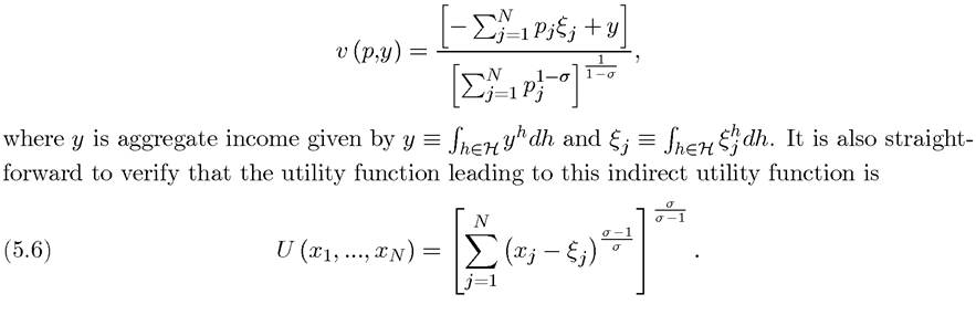
Preferences closely related to the CES preferences presented in this example will play a special role not only in aggregation but also in ensuring balanced growth in neoclassical growth models.

The converse to Theorem 5.2 is also straightforward; Gorman preferences are not only sufficient for the economy to admit a representative household, but they are also necessary. In particular, if preferences do not take the Gorman form (with the same b (p) for all households), then there will exist a specific redistribution of income that will change demands and thus the economy cannot admit a representative household.³ Since this result is not central to our focus, I will not state it formally and provide a proof.

In addition to the aggregation result in Theorem 5.2, Gorman preferences also imply the existence of a normative representative household, in the sense that not only there exists a representative household whose maximization problem will generate the relevant aggregate demands, but also the utility function of this household can be used for welfare analysis. More

₃

³Naturally, we can obtain a broader class of preferences for which aggregate behavior can be represented as if it resulted from the maximization problem of a single representative household if we are willing to restrict attention to specific distribution of income (wealth) across households.

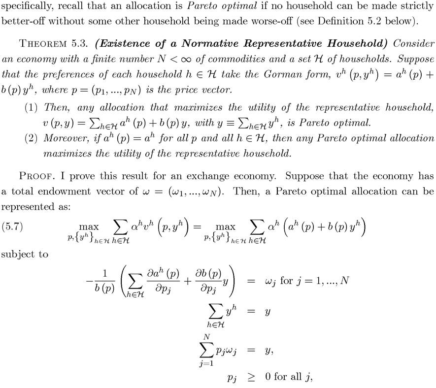
where₍ are nonnegative Pareto weights with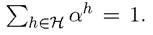The first set of con­

straints use Roy’s identity to express the total demand for good j and set it equal to the supply of good j, which is the endowment ωj. The second equation defines total income as the sum of the income of the households. The third equation makes sure that total income in the economy is equal to the value of the endowments. The third set of constraints requires that all prices are nonnegative.

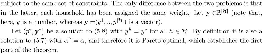
Now compare the maximization problem (5.7) to the following problem:

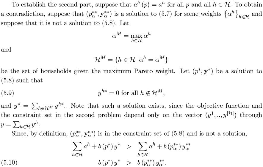
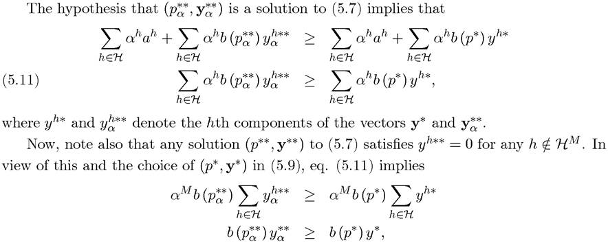
which contradicts eq. (5.10), and establishes that, under the stated assumptions, any Pareto optimal allocation maximizes the utility of the representative household. ?

5.3.