Setting Monetary Policy Targets

We described the tools of monetary policy in Section 14.2. But how do policymak- ^setting of monetary ers use these tools in practice? In this section, we show the main considerations for ^poliC^{y targets}.

Targeting the Federal Funds Rate

In conducting monetary policy, the Fed has certain goals, or ultimate targets, such as price stability and stable economic growth. In trying to reach these goals, the Fed can use the monetary policy tools, or instruments, that we've discussed: reserve requirements, the discount rate, the interest rate on reserves, and especially open-market operations. The problem the Fed faces is how to use the instruments that it controls directly, particularly open-market operations, to achieve its goals. Because there are several steps between open-market operations and the ultimate behavior of prices and economic activity—and because these steps often can't be predicted accurately—the Fed uses intermediate targets to guide monetary policy. Intermediate targets, also sometimes called indicators, are macroeconomic variables that the Fed cannot control directly but can influence fairly predictably, and that in turn are related to the goals the Fed is trying to achieve.

Historically, the most frequently used intermediate targets have been mone­tary aggregates, such as M1 and M2, and short-term interest rates, such as the fed funds rate. By using open-market operations, the Fed can directly control the level of the monetary base, which influences the monetary aggregates. Fluctuations in the money supply in turn affect interest rates, at least temporarily, by causing the LM curve to shift. Neither monetary aggregates nor short-term interest rates are important determinants of economic welfare in and of themselves, but both influ­ence the state of the macroeconomy.

At various times the Fed has guided monetary policy by attempting to keep either monetary growth rates or short-term interest rates in or near pre-established target ranges. Note that, although the Fed may be able to stabilize one or the other of these variables, it cannot target both simultaneously. For example, suppose that the Fed were trying to target both the money supply and the fed funds rate and that the pre-established target ranges called for an increase in both variables. How could the Fed meet these targets simultaneously? If it raised the monetary base to raise the money supply, in the short run the increase in money supply would shift the LM curve down and to the right, which would lower rather than raise the fed funds rate. Alternatively, if the Fed lowered the monetary base to try to increase the fed funds rate, the money supply would fall instead of rising, as required. Thus, in general, the Fed cannot simultaneously meet targets for both interest rates and the money supply, unless those targets are set to be consistent with each other.

In recent years the Fed has typically downplayed monetary aggregates and focused on stabilizing the fed funds rate at a target level. Figure 14.5 shows a

FIGUREJ4.5

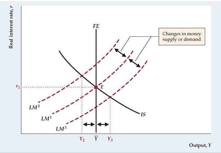
situation in which this strategy is useful. When the LM curve is LM¹, the economy is at full-employment equilibrium at point E, with output at Y and a real interest rate of r₁. Suppose that most of the shocks hitting the economy are nominal shocks, including shocks to money supply and to money demand. Without intervention by the Fed, these nominal shocks cause the LM curve to shift between LM² and LM³, leading aggregate demand to shift erratically between Y₂ and Y₃.

The Fed could reduce the instability caused by nominal shocks by using mon­etary policy to hold the real interest rate at r₁.^[262] In other words, whenever the LM curve shifted up to LM², the Fed could increase the money supply to restore the LM curve to LM¹; similarly, shifts of the LM curve to LM³ could be offset by reduc­tions in the money supply to return the LM curve to LM¹. In this case stabilizing the intermediate target, the interest rate, also would stabilize output at its full­employment level. For interest rate targeting to be a good strategy, however, nomi­nal shocks, that is, shocks to the LM curve, must be the main source of instability.

When the Fed decided to target the fed funds rate in the late 1980s, some econ­omists worried that the central bank was returning to a flawed policy that contrib­uted to the large rise in inflation in the 1960s and 1970s. But Fed policymakers argued that the policy flaw was not the use of the fed funds rate as an intermedi­ate target per se, but the Fed's failure to change its target for the fed funds rate in a timely manner.

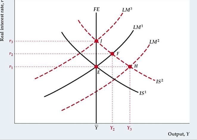
Suppose, for example, that a shock hits the economy that shifts the IS curve to the right; a sudden increase in foreign demand for exported goods is one possibility. How should the Fed respond? Figure 14.6 illustrates this situation. In the graph, suppose that before the shock, the economy is in general equilibrium at point E, where the initial IS curve, IS¹, intersects the initial LM curve, LM¹, so the initial equilibrium real interest rate is r₁ and the level of output is Y. The increase in export demand causes the IS curve to shift up and to the right to IS². If the Fed were to keep the LM curve unchanged at LM¹, then, as shown by point F, output would rise to Y₂ and the real interest rate would rise to r₂ in the short run, and the price level would rise in the long run.

FIGUREJ4.6

Interest rate targeting when an /S shock occurs

The figure shows an economy that starts at point E and experiences a shock that shifts the IS curve up and to the right. A Fed policy of not changing the LM curve leads to higher output at Y₂ and a higher real inter­est rate at r₂ in the short run (point F), and the price level would rise in the long run. A Fed pol­icy of maintaining the real interest rate at r₁ by increasing the money supply causes the LM curve to shift to LM², increasing output to Y₃ in the short run (point H) and raising the price level in the long run. A Fed policy of raising the real interest rate to r₃ by reducing the money sup­ply and shifting the LM curve to LM³ is the only way to maintain full employment (point J) in the short run and not increase the price level in the long run.

To summarize, our analysis in Figs. 14.5 and 14.6 shows that when there are shocks to the LM curve, the Fed can stabilize the economy by setting a fixed real interest rate. But if there are shocks to the IS curve, the Fed needs to modify its target for the interest rate, or else its policy is destabilizing.

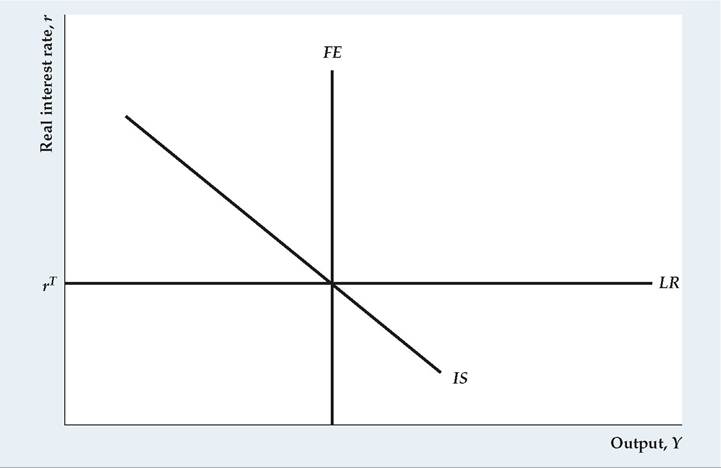
If the Fed targets the real interest rate, then it is useful to modify the LM curve. Rather than having the LM slope upward as in our previous graphs, we could instead directly show the Fed's policy as represented by a horizontal line in the IS-LM diagram (Figure 14.7), which we will call the LR curve. In the graph, the target real interest rate is denoted r^T. The Fed uses open-market operations to hit this target real interest rate on a day-to-day basis and allows the money supply to change to whatever level is necessary to attain this target.

In setting monetary policy using the LR curve, the Fed now must think about what real interest rate is desirable for the economy rather than what nominal money supply is needed. Consider the Fed's response to a shock to the IS curve, which we considered in Fig. 14.6. In that situation, we noted that the Fed should modify its target for the real federal funds rate to keep the economy at its full­employment equilibrium without causing a change in the price level in the long run. Thus the Fed must be flexible in setting its real federal funds rate target, r^τ, constantly monitoring the economy to see if the IS curve might have shifted. To see how the Fed can change its fed funds target to promote economic stability and low inflation, see the section on the Taylor Rule.

One advantage of targeting the real interest rate and using the LR curve is that shocks to money demand are automatically offset. An increase in money demand caused by some shock to the economy is automatically matched by an increase in money supply, and the real interest rate remains unchanged.

FIGUREJ4.7

The LR curve

The horizontal LR curve replaces the LM curve in a situation in which the Fed targets the real inter­est rate. The Fed allows the money supply to change in the short run to hit its target for the real interest rate.

Monetary Policy with Abundant Reserves

In the aftermath of the financial crisis, the Fed changed its method of engaging in monetary policy on a day-to-day basis. Because quantitative easing had increased the supply of reserves to a very high level, the federal funds rate was determined more by the interest rate on reserves rather than the supply and demand for reserves. This new abundant-reserves regime is illustrated in Figure 14.8.

In Fig. 14.8, the primary credit discount rate is d. The fed funds rate would not rise above d because if it did, banks in good condition that want additional reserves would borrow reserves from the Fed at the primary credit discount rate rather than borrow from other banks in the fed funds market. Therefore, the demand for fed funds by banks in good condition would fall to zero if the fed funds rate were even a tiny amount higher than the primary credit discount rate, d.

In the figure, IORB is the rate of interest on reserve balances. If the fed funds rate were to fall below IORB, then banks could earn virtually unlimited arbitrage profits by borrowing reserves at the fed funds rate and earning the IORB rate on those reserves. The possibility of virtually unlimited arbitrage profits for banks if the fed funds rate were to fall below IORB makes the demand for reserves infi­nitely elastic when the fed funds rate equals the IORB rate; thus, the demand curve become horizontal when the fed funds rate equals the IORB rate.^[265]

FIGUREJ4.8

The Reserves Market with Abundant Reserves.

When bank reserves are abundant, the supply of reserves, S, intersects the demand for reserves, D, on the horizontal portion of the demand curve at the interest rate on reserves. As a result, the equilibrium federal funds rate equals the interest rate on reserves.

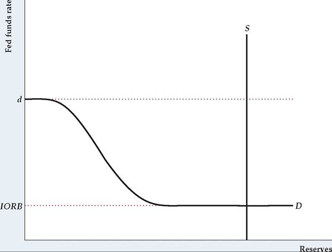
The vertical line labeled S is the supply curve of reserves, which is determined by the Fed. The Fed chooses the monetary base, MB, and knows the amount of cur­rency, C, in circulation. The supply of reserves equals MB - C. Given that d is the maximum level of the fed funds rate and IORB is the minimum level, banks' demand for reserves is given by the curve labeled D. Prior to 2008, the relevant portion of the demand curve was the downward-sloping part. But after the Fed engaged in quan­titative easing in a major way, the S line moved so far to the right that it intersected the D curve on its horizontal segment, where the fed funds rate equals IORB.

With the equilibrium in the economy like that depicted in Fig. 14.8, small move­ments of the supply curve do not affect the fed funds rate. So, if the Fed engages in quantitative easing to move the supply curve to the right, there is no change to the fed funds rate, but the open-market purchases of long-term bonds may affect the market for long-term securities, so long-term interest rates may decline. Similarly, quantitative tightening, in which the Fed sells securities in the open market, have no impact on short-term interest rates, but might raise long-term interest rates.

If the Fed wants to raise interest rates in the situation shown in Fig. 14.8, it can do so by raising the IORB rate, as Figure 14.9 shows. The original equilibrium is at point A, with the fed funds rate equal to IORB₀ and the amount of reserves at R*. The Fed increases the interest rate on reserves from IORB₀ to IORB₁. Usually, the Fed raises the discount rate at the same time that it raises the interest rate on reserves, so this is shown by a rise in the discount rate from d₀ to d₁. In equilib­rium, the quantity of reserves in the market remains unchanged at R* and the federal funds rate rises to IORB₁.

When the Fed raises the interest rate on reserves, it often reduces the supply of reserves at the same time, which would be depicted as a shift to the left of the

FIGUREJ4.9

A Rise in the Interest Rate on Reserves when Reserves Are Abundant

When bank reserves are abundant, an increase in the interest rate on reserves from IORB₀ to IORB₁ leads to a rise in the equilibrium federal funds rate.

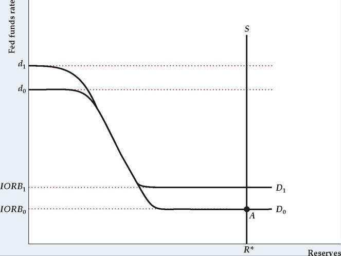
supply curve, S. Doing so would not have any impact on the federal funds rate (as long as the equilibrium between demand and supply of reserves remains on the horizontal part of the demand curve) but would reduce the equilibrium amount of reserves. To keep things simple, we have not shown this effect in Fig. 14.9, but that is an easy effect to add to the diagram.

14.4