The Demand for Labor
Discuss factors that affect the demand for labor.
We have shown that the amount of output produced by a country, or by a firm, depends both on productivity and the quantities of inputs used in the production process.
In Section 3.1 our focus was on productivity—its measurement and factors such as supply shocks that cause it to change. In this section, we examine what determines the quantities of inputs that producers use.Recall that the two most important inputs are capital and labor. The capital stock in an economy changes over time as a result of investment by firms and the scrapping of worn-out or obsolete capital. However, because the capital stock is long-lived and has been built up over many years, new investment and the scrapping of old capital only slowly have a significant effect on the overall quantity of capital available. Thus, for analyses spanning only a few quarters or years, economists often treat the economy's capital stock as fixed. For now we follow this practice and assume a fixed capital stock. In taking up long-term economic growth in Chapter 6, we drop this assumption and examine how the capital stock evolves over time.
In contrast to the amount of capital, the amount of labor employed in the economy can change fairly quickly. For example, firms may lay off workers or ask them to work overtime without much notice. Workers may quit or decide to enter the work force quickly. Thus year-to-year changes in production often can be traced to changes in employment. To explain why employment changes, for the remainder of this chapter we focus on how the labor market works, using a supply and demand approach. In this section we look at labor demand, and in Section 3.3 we discuss factors affecting labor supply.
As a step toward understanding the overall demand for labor in the economy, we consider how an individual firm decides how many workers to employ.
To keep things simple for the time being, we make the following assumptions:1. Workers are all alike. We ignore differences in workers' aptitudes, skills, ambitions, and so on.
2. Firms view the wages of the workers they hire as being determined in a competitive labor market and not set by the firms themselves. For example, a competitive firm in Cleveland that wants to hire machinists knows that it must pay the going local wage for machinists if it wants to attract qualified workers. The firm then decides how many machinists to employ.
3. In making the decision about how many workers to employ, a firm's goal is to earn the highest possible level of profit (the value of its output minus its costs of production, including taxes). The firm will demand the amount of labor that maximizes its profit.
To figure out the profit-maximizing amount of labor, the firm must compare the costs and benefits of hiring each additional worker. The cost of an extra worker is the worker's wage, and the benefit of an extra worker is the value of the additional goods or services the worker produces. As long as the benefits of additional labor exceed the costs, hiring more labor will increase the firm's profits. The firm will continue to hire additional labor until the benefit of an extra worker (the value of extra goods or services produced) equals the cost (the wage).
The Marginal Product of Labor and Labor Demand: An Example
Let's make the discussion of labor demand more concrete by looking at The Clip Joint, a small business that grooms dogs. The Clip Joint uses both capital, such as clippers, tubs, and brushes, and labor to produce its output of groomed dogs.
The production function that applies to The Clip Joint appears in Table 3.2. For given levels of productivity and the capital stock, it shows how The Clip Joint's daily output of groomed dogs, column (2), depends on the number of workers employed, column (1). The more workers The Clip Joint has, the greater its daily output.
The MPN of each worker at The Clip Joint is shown in column (3). Employing the first worker raises The Clip Joint's output from 0 to 11, so the MPN of the first worker is 11. Employing the second worker raises The Clip Joint's output from 11 to 20, an increase of 9, so the MPN of the second worker is 9; and so on. Column (3) also shows that, as the number of workers at The Clip Joint increases, the MPN falls so that labor at The Clip Joint has diminishing marginal productivity. The more workers there are on the job, the more they must share the fixed amount of capital (tubs, clippers, brushes), and the less benefit there is to adding yet another worker.
The marginal product of labor measures the benefit of employing an additional worker in terms of the extra output produced. A related concept, the marginal revenue product of labor (MRPN) measures the benefit of employing an additional worker in terms of the extra revenue produced. To calculate the MRPN, we need to know the price of the firm's output. If The Clip Joint receives $30 for each dog it grooms, the MRPN of the first worker is $330 per day (11 additional dogs groomed per day at $30 per grooming). More generally, the marginal revenue product of an additional worker equals the price of the firm's output, P, times the extra output gained by adding the worker, MPN:
MRPN = P ? MPN. (3.3)
TABLE 3.2
The Clip Joint’s Production Function
| (1) Number of workers, N | (2) Number of dogs groomed, Y | (3) Marginal product of labor, MPN | (4) Marginal revenue product of labor, MRPN = MPN ? P (when P = $30 per grooming) |
| 0 | 0 | ||
| 11 | $330 | ||
| 1 | 11 | ||
| 9 | $270 | ||
| 2 | 20 | ||
| 7 | $210 | ||
| 3 | 27 | ||
| 5 | $150 | ||
| 4 | 32 | ||
| 3 | $90 | ||
| 5 | 35 | ||
| 1 | $30 | ||
| 6 | 36 |
At The Clip Joint the price of output, P, is $30 per grooming, so the MRPN of each worker, column (4), equals the MPN of the worker, column (3), multiplied by $30.
Now suppose that the wage, W, that The Clip Joint must pay to attract qualified workers is $240 per day. (We refer to the wage, W, when measured in the conventional way in terms of today's dollars, as the nominal wage.) How many workers should The Clip Joint employ to maximize its profits? To answer this question, The Clip Joint compares the benefits and costs of employing each additional worker. The benefit of employing an additional worker, in dollars per day, is the worker 's marginal revenue product, MRPN. The cost of an additional worker, in dollars per day, is the nominal daily wage, W.
Table 3.2 shows that the MRPN of the first worker is $330 per day, which exceeds the daily wage of $240, so employing the first worker is profitable for The Clip Joint. Adding a second worker increases The Clip Joint's profit as well because the MRPN of the second worker ($270 per day) also exceeds the daily wage. However, employing a third worker reduces The Clip Joint's profit because the third worker's MRPN of $210 per day is less than the $240 daily wage. Therefore, The Clip Joint's profit-maximizing level of employment at $240/day—equivalently, the quantity of labor demanded by The Clip Joint—is two workers.
In finding the quantity of labor demanded by The Clip Joint, we measured the benefits and costs of an extra worker in nominal, or dollar, terms. If we measure the benefits and costs of an extra worker in real terms, the results would be the same. In real terms the benefit to The Clip Joint of an extra worker is the number of extra groomings that the extra worker provides, which is the marginal product of labor, MPN. The real cost of adding another worker is the real wage, which is the wage measured in terms of units of output. Algebraically, the real wage, w, equals the nominal wage, W, divided by the price of output, P.
In this example the nominal wage, W, is $240 per day and the price of output, P, is $30 per grooming, so the real wage, w, equals ($240 per day)/($30 per grooming), or 8 groomings per day.
To find the profit-maximizing level of employment, The Clip Joint compares this real cost of an additional worker with the real benefit of an additional worker, the MPN. The MPN of the first worker is 11 groomings per day, which exceeds the real wage of 8 groomings per day, so employing this worker is profitable. The second worker also should be hired, as the second worker's MPN of 9 groomings per day also exceeds the real wage of 8 groomings per day. However, a third worker should not be hired because the third worker's MPN of 7 groomings per day is less than the real wage. The quantity of labor demanded by The Clip Joint is therefore two workers, which is the same result we got when we compared costs and benefits in nominal terms.This example shows that, when the benefit of an additional worker exceeds the cost of an additional worker, the firm should increase employment so as to maximize profits. Similarly, if at the firm's current employment level the benefit of the last worker employed is less than the cost of the worker, the firm should reduce employment. For example, if The Clip Joint currently employed three workers, the MRPN of the third worker is $210, which is less than the nominal wage of $240, so the firm should fire one worker. Summary table 2 compares benefits and costs of additional labor in both real and nominal terms. In the choice of the profitmaximizing level of employment, a comparison of benefits and costs in either real or nominal terms is equally valid.
A Change in the Wage
The Clip Joint's decision to employ two workers was based on a nominal wage of $240 per day. Now suppose that for some reason the nominal wage needed to attract qualified workers drops to $180 per day. How will the reduction in the nominal wage affect the number of workers that The Clip Joint wants to employ?
To find the answer, we can compare costs and benefits in either nominal or real terms. Let's make the comparison in real terms. If the nominal wage drops to $180 per day while the price of groomings remains at $30, the real wage falls to ($180 per day)/($30 per grooming), or 6 groomings per day. Column (3) of Table 3.2 shows that the MPN of the third worker is 7 groomings per day, which is now greater than the real wage.
Thus, at the lower wage, expanding the quantity of labor demanded from two to three workers is profitable for The Clip Joint. However, the firm will not hire a fourth worker because the MPN of the fourth worker (5 groomings per day) is less than the new real wage (6 groomings per day).This example illustrates a general point about the effect of the real wage on labor demand: All else being equal, a decrease in the real wage raises the amount of labor demanded. Similarly, an increase in the real wage decreases the amount of labor demanded.
The Marginal Product of Labor and the Labor Demand Curve
Using The Clip Joint as an example, we showed the negative relationship between the real wage and the quantity of labor that a firm demands. Figure 3.5 shows in more general terms how the link between the real wage and the quantity of labor demanded is determined. The amount of labor, N, is on the horizontal axis. The MPN and the real wage, both of which are measured in goods per unit of labor, are on the vertical axis. The downward-sloping curve is
SUMMARY 2
Comparing the Benefits and Costs of Changing the Amount of Labor
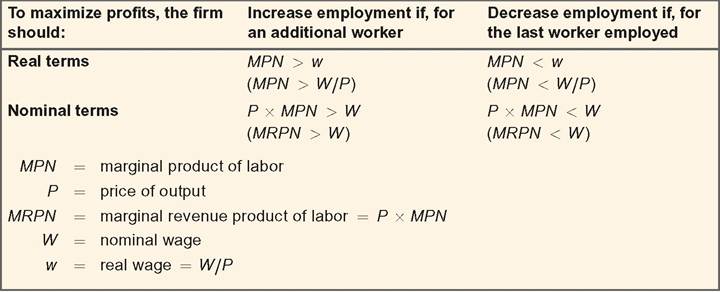
FIGURE 3.5
The determination of labor demand
The amount of labor demanded is determined by locating the point on the MPN curve at which the MPN equals the real wage rate; the amount of labor corresponding to that point is the amount of labor demanded. For example, when the real wage is w*, the MPN equals the real wage at point A and the quantity of labor demanded is N *. The labor demand curve, ND, shows the amount of labor demanded at each level of the real wage. The labor demand curve is identical to the MPN curve. product of labor for the MPN curve.[38] Like the MPN curve, the labor demand curve slopes downward, indicating that the quantity of labor demanded falls as the real wage rises.
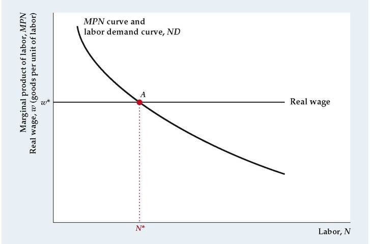
the MPN curve; it relates the marginal product of labor, MPN, to the amount of labor employed by the firm, N. The MPN curve slopes downward because of the diminishing marginal productivity of labor. The horizontal line represents the real wage firms face in the labor market, which the firms take as given. Here, the real wage is w*.
For any real wage, w*, the amount of labor that yields the highest profit (and therefore the amount of labor demanded) is determined at point A, the intersection of the real-wage line and the MPN curve. At A the quantity of labor demanded is N *. Why is N * a firm's profit-maximizing level of labor input? At employment levels less than N *, the marginal product of labor exceeds the real wage (the MPN curve lies above the real-wage line); thus, if the firm's employment is initially less than N *, it can increase its profit by expanding the amount of labor it uses. Similarly, if the firm's employment is initially greater than N *, the marginal product of labor is less than the real wage (MPN < w*) and the firm can raise profits by reducing employment. Only when employment equals N * will the firm be satisfied with the number of workers it has. More generally, for any real wage, the profit-maximizing amount of labor input—labor demanded—corresponds to the point at which the MPN curve and the real- wage line intersect.
The graph of the relationship between the amount of labor demanded by a firm and the real wage that the firm faces is called the labor demand curve. Because the MPN curve also shows the amount of labor demanded at any real wage, the labor demand curve is the same as the MPN curve, except that the vertical axis measures the real wage for the labor demand curve and measures the marginal
This labor demand curve is more general than that in the example of The Clip Joint in a couple of ways that are worth mentioning. First, we referred to the demand for labor and not specifically to the demand for workers, as in The Clip Joint example. In general, labor, N, can be measured in various ways—for example, as total hours worked, total weeks worked, or the number of employees—depending on the application. Second, although we assumed in the example that The Clip Joint had to hire a whole number of workers, the labor demand curve shown in Fig. 3.5 allows labor, N, to have any positive value, whole or fractional. Allowing N to take any value is sensible because people may work fractions of an hour.
Factors That Shift the Labor Demand Curve
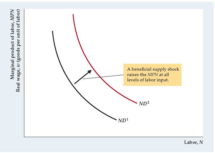
Because the labor demand curve shows the relation between the real wage and the amount of labor that firms want to employ, changes in the real wage are represented as movements along the labor demand curve. Changes in the real wage do not cause the labor demand curve to shift. The labor demand curve shifts in response to factors that change the amount of labor that firms want to employ at any given level of the real wage. For example, we showed earlier in this chapter that beneficial, or positive, supply shocks are likely to increase the MPN at all levels of labor input and that adverse, or negative, supply shocks are likely to reduce the MPN at all levels of labor input. Thus a beneficial supply shock shifts the MPN curve upward and to the right and raises the quantity of labor demanded at any given real wage; an adverse supply shock does the reverse.
The effect of a supply shock on The Clip Joint's demand for labor can be illustrated by imagining that the proprietor of The Clip Joint discovers that playing classical music soothes the dogs. It makes them more cooperative and doubles the number of groomings per day that the same number of workers can produce. This technological improvement gives The Clip Joint a new production function, as described in Table 3.3. Note that doubling total output doubles the MPN at each employment level.
The Clip Joint demanded two workers when faced with the original production function (Table 3.2) and a real wage of 8 groomings per day. Table 3.3 shows that the productivity improvement increases The Clip Joint's labor demand at the given real wage to four workers, because the MPN of the fourth worker (10 groomings per day) now exceeds the real wage. The Clip Joint will not hire a fifth worker, however, because this worker's MPN (6 groomings per day) is less than the real wage.
The effect of a beneficial supply shock on the labor demand curve is shown in Figure 3.6. The shock causes the MPN to increase at any level of labor input, so the MPN curve shifts upward and to the right. Because the MPN and labor demand curves are identical, the labor demand curve also shifts upward and to the right, from ND1 to ND2 in Fig. 3.6. When the labor demand curve is ND2, the firm hires more workers at any real wage level than when the labor demand curve is ND1. Thus worker productivity and the amount of labor demanded are closely linked.
TABLE 3.3
The Clip Joint's Production Function After a Beneficial Productivity Shock
| (1) Number of workers, N | (2) Number of dogs groomed, Y | (3) Marginal product of labor, MPN | (4) Marginal revenue product of labor, MRPN = MPN ? P (when P = $30 per grooming) |
| 0 | 0 | ||
| 22 | $660 | ||
| 1 | 22 | ||
| 18 | $540 | ||
| 2 | 40 | ||
| 14 | $420 | ||
| 3 | 54 | bgcolor=white>||
| 10 | $300 | ||
| 4 | 64 | ||
| 6 | $180 | ||
| 5 | 70 | ||
| 2 | $60 | ||
| 6 | 72 |
Another factor that may affect labor demand is the size of the capital stock. Generally, an increase in the capital stock, K—by giving each worker more machines or equipment to work with—raises workers' productivity and increases the MPN at any level of labor. Hence an increase in the capital stock will cause the
| SUMMARY 3 | ||
| Factors That Shift | he Aggregate Labor Demand Curve | |
| An increase in | Causes the labor demand curve to shift | Reason |
| Productivity | Right | Beneficial supply shock increases MPN and shifts MPN curve up and to the right. |
| Capital stock | Right | Higher capital stock increases MPN and shifts MPN curve up and to the right. |
labor demand curve to shift upward and to the right, raising the amount of labor that a firm demands at any particular real wage.[39]
Aggregate Labor Demand
So far we have focused on the demand for labor by an individual firm, such as The Clip Joint. For macroeconomic analysis, however, we usually work with the concept of the aggregate demand for labor, or the sum of the labor demands of all the firms in an economy.
Because the aggregate demand for labor is the sum of firms' labor demands, the factors that determine the aggregate demand for labor are the same as those for an individual firm. Thus the aggregate labor demand curve looks the same as the labor demand curve for an individual firm (Fig. 3.5). Like the firm's labor demand curve, the aggregate labor demand curve slopes downward, showing that an increase in the economywide real wage reduces the total amount of labor that firms want to use. Similarly, a beneficial supply shock or an increase in the aggregate capital stock shifts the aggregate labor demand curve upward and to the right; an adverse supply shock or a drop in the aggregate capital stock shifts it downward and to the left. The factors affecting aggregate labor demand are listed for convenience in Summary table 3.
3.3