How Much Does the Economy Produce? The Production Function
Dιscuss production function properties and changes.
Every day the business news reports many economic variables that influence the economy's performance—the rate of consumer spending, the value of the dollar, the gyrations of the stock market, the growth rate of the money supply, and so on.
All of these variables are important. However, no determinant of economic performance and living standards is more basic than the economy's physical capacity to produce goods and services. If an economy's factories, farms, and other businesses all shut down for some reason, other economic factors wouldn't mean much.What determines the quantity of goods and services that an economy can produce? A key factor is the quantity of inputs—such as capital goods, labor, raw materials, land, and energy—that producers in the economy use. Economists refer to inputs to the production process as factors of production. All else being equal, the greater the quantities of factors of production used, the more goods and services are produced.
Of the various factors of production, the two most important are capital (factories, machines, software, and intellectual property, for example) and labor (workers). Hence we focus on these two factors in discussing an economy's capacity to produce goods and services. In modern economies, however, output often responds strongly to changes in the supply of other factors, such as energy or raw materials. Later in this chapter, the Application "Output, Employment, and the Real Wage During Oil Price Shocks," discusses the effects of a disruption in oil supplies on the economy.
The quantities of capital and labor (and other inputs) used in production don't completely determine the amount of output produced. Equally important is how effectively these factors are used. For the same stocks of capital and labor, an economy with superior technologies and management practices, for example, will produce a greater amount of output than an economy without those strengths.
The effectiveness with which capital and labor are used may be summarized by a relationship called the production function. The production function is a mathematical expression relating the amount of output produced to quantities of capital and labor utilized. A convenient way to write the production function is

where
Y = real output produced in a given period of time;
A = a number measuring overall productivity;
K = the capital stock, or quantity of capital used in the period;
N = the number of workers employed in the period;
F = a function relating output Y to capital K and labor N.
The production function in Eq. (3.1) applies both to an economy as a whole (where Y, K, and N refer to the economy's output, capital stock, and number of workers, respectively) and to an individual firm, in which case Y, K, and N refer to the firm's output, capital, and number of workers, respectively.
According to Eq. (3.1), the amount of output Y that an economy (or firm) can produce during any period of time depends on the size of the capital stock K and the number of workers N. The symbol A in Eq. (3.1), which multiplies the function F (K, N), is a measure of the overall effectiveness with which capital and labor are used. We refer to A as total factor productivity, or simply productivity. Note that, for any values of capital and labor, an increase in productivity of, say, 10% implies a 10% increase in the amount of output that can be produced. Thus increases in productivity, A, correspond to improvements in production technology or to any other change in the economy that allows capital and labor to be utilized more effectively.
Application
TABLE 3.1
The Production Function of the EU-28, 2005-2014
| Year | (1) Real GDP (Y) in 2010 prices Million EUR | (2) Real Capital Stock (K) in 2010 prices Million EUR | (3) Labor, N (millions of workers) | (4) A = Y∕(K0>33N067) | (5) Growth in A (% change in A) |
| 2005 | 12,230 | 2660 | 208 | 25.35 | — |
| 2006 | 12,647 | 2848 | 212 | 25.32 | 0.12% |
| 2007 | 13,037 | 3031 | 216 | 25.55 | 0.91% |
| 2008 | 13,103 | 2980 | 218 | 25.36 | - 0.74% |
| 2009 | 12,527 | 2478 | 214 | 26.1 | 2.92% |
| 2010 | 12,789 | 2613 | 212 | 26.33 | 0.88% |
| 2011 | 13,011 | 2696 | 212 | 26.51 | 0.68% |
| 2012 | 12,943 | 2539 | 211 | 26.99 | 1.8% |
| 2013 | 12,956 | 2513 | 210 | 27.19 | 0.74% |
| 2014 | 13,127 | 2576 | 213 | 27.08 | - 0.40% |
Source: Real GDR capital stock, and labor force figures are from the Eurostat Database website, htt-p://ec.europa.eu/eurostat/data/database.
Researchers of the EU Economic Policy Committee empirically describe the relationship between output and inputs in the European Union through the following production function:2

The production function in Eq. (3.2) is a specific example of the general production function in Eq. (3.1), in which we set the general function F(K, N) equal to K0.33N0.67 (Note that this production function contains exponents; if you need to review the properties of exponents, see Appendix A, Section A.6.) Equation (3.2) shows how output, Y, relates to the use of factors of production, capital, K, and labor, N, and to productivity, A, in the European Union.
Table 3.1 shows data on these variables for the 28 EU nations from 2005 to 2014. Columns (1), (2), and (3) show real output or GDP, capital stock, and labor for each year. Real GDP and the capital stock are measured in millions of 2010 euros, and labor is measured in millions of employed workers. Column (4) shows the EU-28 growth rates for production during the same period. It is 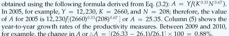
[1]This is called a Cobb-Douglas production function. Cobb-Douglas production functions take the form Y = AKaN 1-a. The parameters a and 1 — a in the Cobb-Douglas production function correspond to the production factor elasticity of labor and capital, respectively. Observing the actual shares of income received by capital and labor provides a way of estimating the parameter a.
An examination of the productivity growth rates (A) in Table 3.1 shows that growth can vary substantially over different periods. As a result of the global financial crisis, productivity took a deep dive in 2008 but showed significant signs of recovery in 2009. Again, the European debt crisis left its marks on productivity in 2014, where A declined by 0.4%.
This may indicate that productivity declines during times of recession and rises during times of economic recovery. But this premise is quite controversial. We return to this issue in Part 3 of this book. The main reason for gauging productivity growth is because it impacts GDP per capita and, hence, standards of living. Chapter 6 details the relationship between productivity and living standards.The Shape of the Production Function
The production function in Eq. (3.1) can be shown graphically. The easiest way to graph it is to hold both total factor productivity and one of the two factors of production, either capital or labor, constant and then graph the relationship between output and the other factor.3 Suppose that we use the U.S. production function for the year 2020 and hold labor N at its actual 2020 value of 157.5 million workers (see Table 3.1). We also use the actual 2020 value of 25.99 for A. The production function Eq. (3.2) becomes

This relationship is graphed in Figure 3.1, with capital stock K on the horizontal axis and output Y on the vertical axis. With labor and productivity held at their 2020 values, the graph shows the amount of output that could have been produced in that year for any value of the capital stock. Point A on the graph shows the situation that actually occurred in 2020: The value of the capital stock ($23,539 billion) appears on the horizontal axis, and the value of real GDP ($18,385 billion) appears on the vertical axis.
The U.S. production function graphed in Fig. 3.1 shares two properties with most production functions:
1. The production function slopes upward from left to right. The slope of the production function reveals that, as the capital stock increases, more output can be produced.
2. The slope of the production function becomes flatter from left to right. This property implies that although more capital always leads to more output, it does so at a decreasing rate.
Before discussing the economics behind the second property of the production function, we can illustrate it numerically, using Fig. 3.1. Suppose that we are initially at point B, where the capital stock is $2000 billion. Adding $1000 billion in capital moves us to point C, where the capital stock is $3000 billion. How much extra output has this expansion in capital provided? The difference in output between points B and C is $1135 billion ($9909 billion output at C minus
3To show the relationship among output and both factors of production simultaneously would require a three-dimensional graph.
FIGURE 3.1
The production function relating output and capital
This production function shows how much output the U.S. economy could produce for each level of U.S. capital stock, holding U.S. labor and productivity at 2020 levels. Point A corresponds to the actual 2020 output and capital stock. The production function has diminishing marginal productivity of capital: Raising the capital stock by $1000 billion to move from point B to point C raises output by $1135 billion, but adding another $1000 billion in capital to go from point C to point D increases output by only $893 billion.
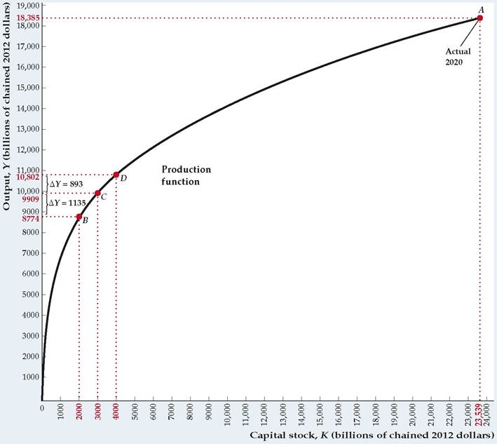
$8774 billion output at B). This extra $1135 billion in output is the benefit from raising the capital stock from $2000 billion to $3000 billion, with productivity and employment held constant.
Now suppose that, starting at C, we add another $1000 billion of capital. This new addition of capital takes us to D, where the capital stock is $4000 billion. The difference in output between C and D is only $893 billion ($10,802 billion output at D minus $9909 billion output at C), which is less than the $1135 billion increase in output between B and C. Thus, although the second $1000 billion of extra capital raises total output, it does so by less than did the first $1000 billion of extra capital.
This result illustrates that the production function rises less steeply between points C and D than between points B and C.The Marginal Product of Capital
The two properties of the production function are closely related to a concept known as the marginal product of capital. To understand this concept, we can start from some given capital stock, K, and increase the capital stock by some amount, ∆ K (other factors held constant). This increase in capital would cause output, Y, to increase by some amount, ∆ Y. The marginal product of capital (MPK) is the increase in output produced that results from a one-unit increase in the capital stock. Because ∆ K additional units of capital permit the production of ∆ Y additional units of output, the amount of additional output produced per additional unit of capital is ∆Y∕∆K. Thus the marginal product of capital is ∆Y∕∆K.
The marginal product of capital, ∆Y∕ ∆K, is the change in the variable on the vertical axis of the production function graph, ∆ Y, divided by the change in the variable on the horizontal axis, ∆ K, which you might recognize as a slope.[32] For small increases in the capital stock, the MPK can be measured by the slope of a line drawn tangent to the production function. Figure 3.2 illustrates this way of measuring the MPK. When the capital stock is 2000, for example, the MPK equals the slope of the line tangent to the production function at point B.[33] We can use the concept of the marginal product of capital to restate the two properties of production functions listed earlier.
1. The marginal product of capital is positive. Whenever the capital stock is increased, more output can be produced. Because the marginal product of capital is positive, the production function slopes upward from left to right.
FIGURE 3.2
The marginal product of capital
The marginal product of capital (MPK) at any point can be measured as the slope of the line tangent to the production function at that point. Because the slope of the line tangent to the production function at point B is greater than the slope of the line tangent to the production function at point D, we know that the MPK is greater at B than at D. At higher levels of capital stock, the MPK is lower, reflecting diminishing marginal productivity of capital.
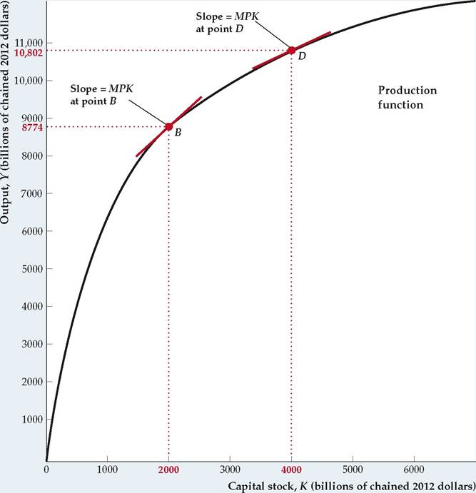
2. The marginal product of capital declines as the capital stock is increased. Because the marginal product of capital is the slope of the production function, the slope of the production function decreases as the capital stock is increased. As Fig. 3.2 shows, the slope of the production function at point D, where the capital stock is 4000, is smaller than the slope at point B, where the capital stock is 2000. Thus the production function becomes flatter from left to right.
The tendency for the marginal product of capital to decline as the amount of capital in use increases is called the diminishing marginal productivity of capital. The economic reason for diminishing marginal productivity of capital is as follows: When the capital stock is low, there are many workers for each machine, and the benefits of increasing capital further are great; but when the capital stock is high, workers already have plenty of capital to work with, and little benefit is to be gained from expanding capital further. For example, in a business firm's call center in which there are many more staff members than workstations (phones and computer terminals), each workstation is constantly being utilized, and the staff must waste time waiting for a free workstation. In this situation, the benefit in terms of increased output of adding extra workstations is high. However, if there are already as many workstations as staff members, so that workstations are often idle and there is no waiting for a workstation to become available, little additional output can be obtained by adding yet another workstation.
The Marginal Product of Labor
In Figs. 3.1 and 3.2 we graphed the relationship between output and capital implied by the 2020 U.S. production function, holding constant the amount of labor. Similarly, we can look at the relationship between output and labor, holding constant both total factor productivity and the quantity of capital. Suppose that we fix capital, K, at its actual 2020 value of $23,539 billion and hold productivity, A, at its actual 2020 value of 25.99 (see Table 3.1). The production function Eq. (3.2) becomes

This relationship is shown graphically in Figure 3.3. Point A, where N = 157.5 million workers and Y = $18,385 billion, corresponds to the actual 2020 values.
The production function relating output and labor looks generally the same as the production function relating output and capital.[34] As in the case of capital, increases in the number of workers raise output but do so at a diminishing rate. Thus the principle of diminishing marginal productivity also applies to labor, and for similar reasons: the greater the number of workers already using a fixed amount of capital and other inputs, the smaller the benefit (in terms of increased output) of adding even more workers.
The marginal product of labor (MPN) is the additional output produced by each additional unit of labor As with the marginal product of capital,
for small increases in employment, the MPN can be measured by the slope of the line tangent to a production function that relates output and labor. In Fig. 3.3, when employment equals 30 million workers, the MPN equals the slope of the
FIGURE 3.3
The production function relating output and labor
This production function shows how much output the U.S. economy could produce at each level of employment (labor input), holding productivity and the capital stock constant at 2020 levels. Point A corresponds to actual 2020 output and employment. The marginal product of labor (MPN) at any point is measured as the slope of the line tangent to the production function at that point. The MPN is lower at higher levels of employment, reflecting diminishing marginal productivity of labor.
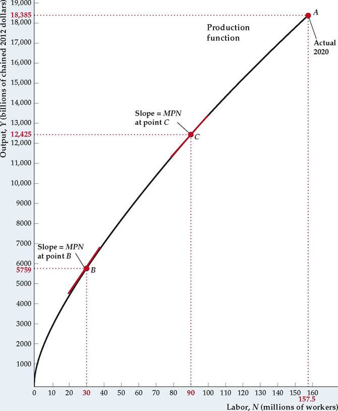
line tangent to the production function at point B; when employment is 90 million workers, the MPN is the slope of the line that touches the production function at point C. Because of the diminishing marginal productivity of labor, the slope of the production function relating output to labor is greater at B than at C, and the production function flattens from left to right.
Supply Shocks
The production function of an economy doesn't usually remain fixed over time. Economists use the term supply shock—or, sometimes, productivity shock—to refer to a change in an economy's production function.[35] A positive, or beneficial, supply
shock raises the amount of output that can be produced for given quantities of capital and labor. A negative, or adverse, supply shock lowers the amount of output that can be produced for each capital-labor combination.
Real-world examples of supply shocks include changes in the weather, such as a drought or an unusually cold winter; inventions or innovations in management techniques that improve efficiency, such as computerized inventory control or statistical analysis in quality control; and changes in government regulations, such as antipollution laws, that affect the technologies or production methods used. Also included in the category of supply shocks are changes in the supplies of factors of production other than capital and labor that affect the amount that can be produced. For example, following the pandemic recession of 2020, shortages of key components (such as semiconductors) led to a shortfall in supplies of automobiles.
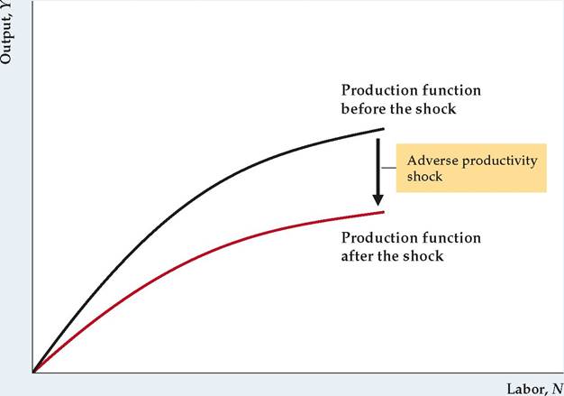
Figure 3.4 shows the effects of an adverse supply shock on the production function relating output and labor. The negative supply shock shifts the production function downward so that less output can be produced for specific quantities of labor and capital. In addition, the supply shock shown reduces the slope of the production function so that the output gains from adding a worker (the marginal product of labor) are lower at every level of employment.[36] Conversely, a beneficial supply shock makes possible the production of more output with given quantities of capital and labor and thus shifts the production function upward.[37]
FIGURE 3.4
An adverse supply shock that lowers the MPN
An adverse supply shock is a downward shift of the production function. For any level of labor, the amount of output that can be produced is now less than before. The adverse shock shown here reduces the slope of the production function at every level of employment.
3.2
More on the topic How Much Does the Economy Produce? The Production Function:
- Step-by-Step Innovations*
- Public enterprises produce public and private goods
- WEALTH DYNAMICS AND ANTIPOVERTY POLICIES
- INTRODUCTION AND OVERVIEW
- MODELING HOUSEHOLD BEHAVIOR: THE COLLECTIVE MODEL
- Unemployment
- Codetermination as an interlocking system
- Basicframework
- The family firm: marriage
- INEQUALITY AND FINANCIAL MARKETS