Unemployment
In his conclusion to The General Theory of Employment, Interest and Money, Keynes wrote that ‘it may be possible by a right analysis of the problem to cure the disease [of unemployment] whilst preserving efficiency and freedom' (Keynes 1936, p.
381). The commitment to high and stable levels of employment of successive UK governments and the actual achievement of low rates of unemployment appeared to support Keynes' proposition, at least as far as unemployment was concerned. Indeed, in the 20 years after the Second World War the unemployment rate rarely exceeded 2%. This ‘golden age', however, ended in the late 1960s and under the influence of two oil shocks during the 1970s and subsequent deflationary policy responses, unemployment in the UK rose to over 3 million by the mid-1980s, i.e. some 11% of the workforce. It again approached 3 million in the early 1990s and, despite a fall in the rate to 4.7% in Summer 2004, the recent world recession has seen the rate rise to over 8% in 2010. It appears that Keynes might have been over-optimistic in his prediction. Indeed, as a recent joint report from the ILO and IMF (2010) has pointed out, there are currently 210 million people unemployed across the world, an increase of 30 million since 2007. They argue that if past recessions are any indicator this will have huge costs to both the unemployed themselves and society as a whole. These costs include lower lifetime earnings, reduced life expectancy and lower educational achievement for their children and an impact on attitudes which will result in less social cohesion. In this chapter we look at the methods of counting the unemployed and at who the unemployed are. We then consider the contribution of economic theory to the issue of unemployment before concluding with an attempt to identify those policies that might lead the economy in the direction of higher employment, especially in view of the global recession following events in the US sub-prime market in late 2007.I Unemployment in the UK
It could be argued that the adoption, after the Second World War, of Keynesian demand-management policies secured nearly two decades of historically low unemployment (see Fig.
23.1). In recent years, however, although government commitment to full employment (first stated in the 1944 White Paper on employment policy) has never been revoked, we no longer appear to have the tools with which to do the job. The traditional reliance on macroeconomic policies as a means of reducing unemployment has largely been replaced by a greater emphasis on microeconomic supply-side measures that take into account the changing nature of the labour market, society and the global economy. Labour market reforms of this type during the 1980s and 1990s and measures such as the ‘New Deal’ of the 1997-2010 Labour government have, however, resulted in a UK unemployment rate that compares favourably with our EU partners. Nevertheless, the UK unemployment rate is still four times as high as it was in the 1950s and 1960s and there is an uneasy feeling that this period of very low unemployment may prove to have been the exception rather than the rule!Before attempting to assess the causes of high unemployment, and to consider what, if anything, can be done, it is important to examine the unemployment statistics themselves to see what light they shed on the issue.
How unemployment is measured
Since January 2003 the UK government’s only official and internationally comparable measure of unemployment has been provided by the Labour Force Survey (LFS). The LFS uses the internationally agreed definition of unemployment recommended by the International Labour Office (ILO). Unemployed people are ‘those without a job who have actively sought work in the last four weeks and are available to start work within the next two weeks, or those who are out of work, but who have found a job but are waiting to start in the next two weeks’.
The LFS samples around 61,000 households in any three-month period and interviews are taken from approximately 120,000 people aged 16 and over. The LFS enables the publication of results for the latest available three months every month.
Results for individual months are not published, however, as they are not thought to be statistically robust. Everyone surveyed is classified as either economically active (in employment or ILO unemployed) or economically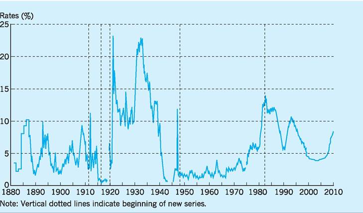
Fig. 23.1 UK unemployment rate, 1881-2010 (excluding school-leavers).
Sources: ONS Labour Market Trends (various); London and Cambridge Economic Service (various).
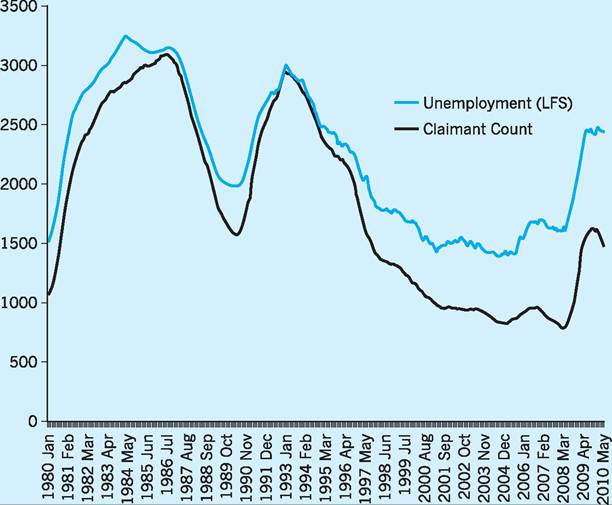
Fig. 23.2 Unemployment and the Claimant Count. Source: ONS (various).
inactive (either wanting a job but not meeting the ILO unemployment criteria, or not wanting a job).
In the three months from May to July 2010 unemployment in the UK stood at 2.47 million. The figure of 2.47 million unemployed represents an unemployment rate of 7.8%. The unemployment rate is calculated by dividing the absolute number of unemployed by the total number of economically active (employed plus unemployed) and expressing this as a percentage.
Claimant Count data, which, in the past, has been used as an alternative measure, calculates unemployment in terms of those claiming unemployment- related benefits (Jobseeker’s Allowance-JSA). Claimant Count data will continue to be published on a monthly basis and provides further information on the labour market. The Claimant Count for August 2010 stood at 1.47 million, a rate of 4.5%.
Figure 23.2 shows both the LFS and Claimant Count measures of unemployment over the period 1980-2010. The two measures show the same broad trend, rising and falling together over the economic cycle. The LFS unemployment figure is usually higher because people who are unemployed are not necessarily eligible for JSA, or may choose not to claim even when eligible. The 16- and 17-year-old group is an example of the former and people over state pension age the latter. The group that has contributed most to the gap is women aged 25-49 who are not eligible for benefit, either because they have not made sufficient National Insurance contributions, or they have too high a level of savings or a partner whose income is too high.
Disaggregating unemployment statistics
Further insight can be gained by breaking down the total unemployment figures into a number of components as follows.
Regional unemployment
The UK has a long history of some regions having a higher than average level of unemployment. Traditionally the explanation of such variations was in terms of the depressed regions being over reliant on declining industries (coal, textiles, shipbuilding) together with limited labour mobility. In 1971, for example, Northern Ireland had an unemployment rate that was double the UK average, whilst in Scotland the rate was 70% above the UK average. In comparison, the South East had an unemployment rate of half the UK average. Declining UK unemployment over the period 1994-2006 saw some narrowing of the regional disparities, although apart from London and the South East the private sector had struggled to create jobs and in the North and the Midlands, the public sector had been the main source of new employment.
The recession since 2007 has reopened the problems for certain regions and cities. At the regional level, Yorkshire and Humberside and the North East have the highest rates of unemployment (9.1% compared to the UK average rate of 7.8% in 2010). However, the regional figures hide considerable differences. Cities in and around the larger industrial conurbations have experienced the largest increases in percentage unemployment, with the continued decline in manufacturing raising percentage unemployment most in cities. The current public sector spending cuts mean that cities with higher percentages of public sector employment will be extremely vulnerable to increased unemployment. Cities with large numbers of people with low skill levels - such as Dudley and Sandwell (12%), Dover (7.4%), Ebbw Vale (12.2%) and Abergavenny - have also experienced higher percentage unemployment. Cities with highly skilled populations and few people with low skill levels, such as Cambridge (2.1%), have fared lot better.
Unemployment and inactivity by gender
Male unemployment rates have always been higher than female rates. The overall UK unemployment rate for the three months to July 2010 was 7.8%, with male unemployment for the same period being 8.5% compared to female unemployment of 7.0%. Additionally, a striking feature has been the rise in male inactivity rates (neither employed nor counted as unemployed) and the fall in female inactivity rates. In June 1976 the female inactivity rate (16-59) was 41.2% and the male inactivity rate (16-64) was 6.4%. By June 2010 the female rate had fallen to 29.3%, but the male rate had risen to 17.0%. This increase in female participation in the labour market arises mainly from married women whose partners are typically working, which more than compensates the fact that the participation rate of single women with children has fallen. The rise in male inactivity rates has mainly involved married men whose partners do not work (or have never worked) and single men. Nickell (2003) finds that the rise in prime-age male inactivity rates is largely accounted for by low- skilled workers claiming incapacity benefit. The weakness of the labour market for unskilled workers plus the relative ease in acquiring incapacity benefit could explain part of this rise in inactivity rates. Recent government measures targeting such males have had limited success. In June 2010 there were over 1.1 million males giving long-term sickness as the reason for inactivity.
As a result of these changes, there has been a growing polarization between work-rich households where both partners work, and work-poor households where no one works. Nickell couples this trend together with growing UK wage dispersion (falling relative wages of unskilled workers) to explain increased poverty in the UK (see Chapter 14 for more details).
Age-related unemployment
The average OECD youth unemployment rate (15-24 years) is about three times that of the adult unemployment rate.
The current global recession has worsened this relative position with the youth rate rising by 6% since 2008, reaching 19% in 2010. The UK figure of 19% in 2010 was high, but less than in some countries such as France (21.4%), Italy (28.9%), Sweden (29.7%) and Spain (41.1%). One notable exception was Germany where an effective apprenticeship scheme and agreements on short-term working had kept the youth unemployment rate at 9%. Evidence suggests that a long period out of work for young workers has a significantly negative impact on their future labour market performance. Table 23.1 indicates that the unemployment rate tends to decline with age; for example only 6.3% of those aged 25-49 years were unemployed in 2010 compared to 32.3% of those aged 16-17 years.However, those older workers who do become unemployed are particularly prone to long spells of unemployment. The long-term unemployed (a year or more) are disproportionately older, disproportionately male and disproportionately low skilled. Such long-term unemployment destroys skills and motivation and is often used by employers as an unfavourable filtering device, leading to the stark statistic that
Table 23.1 UK unemployment rates (%) by age, May-July 2010.
| 16-17 | 18-24 | 25-49 | bgcolor=white>50 and over16-59/64 | ||
| All persons | 32.3 | 17.4 | 6.3 | 4.6 | 8.0 |
| Men | 35.8 | 19.0 | 6.7 | 5.7 | 8.7 |
| Women | 28.9 | 15.5 | 5.9 | 3.2 | 7.1 |
| Source: ONS (various). |
Table 23.2 Percentage of UK unemployed who have been out of work for over a year, May-July 2010.
| 16-17 | 18-24 | 25-49 | 50 and over | 16-59/64 | |
| All persons | 11.0 | 26.3 | 36.0 | 42.9 | 33.2 |
| Men | 12.1 | 32.5 | 42.2 | 44.3 | 37.6 |
| Women | N/a | 17.6 | 27.8 | 39.9 | 24.4 |
| Source: ONS (various). |
those workers who are still unemployed after two years stand only a 50% chance of leaving unemployment for a job within the following year. Table 23.2 indicates that 42.9% of the unemployed aged 50 and over had been unemployed for a year or more, compared to only 26.3% of the unemployed aged 18-24 years. The government’s strategy towards both youth and long-term unemployment in the UK is discussed later in the chapter.
It is worth noting that the fall in the proportion of youths in the labour force over the last 20 years (a result of the low birth rate in the 1970s) may have contributed as much as 0.55 percentage points of the 5.65 percentage points fall in the UK unemployment rate between 1984 and 1998. It was thought unlikely, however, that shifts in the age composition of the labour force would have much effect on the unemployment rate over the first 10 years of the new millennium (Barwell 2000).
Qualifications and unemployment
The demand for low-skilled and poorly educated workers has been declining throughout the OECD since the early 1980s, whereas the demand for skilled workers has outstripped the supply. The overall result is that the employment prospects and wages of poorly educated and unskilled workers have deteriorated relative to those for better educated and skilled workers. Almost 90% of those with a degree or equivalent as their highest qualification were in employment, which compares with only 48% of people with no qualifications. People with higher qualifications are less likely to be unemployed or economically inactive. Similarly the wage gap between men aged 25-49 years with no qualifications and those with a university degree was 61% in 1979, but this gap had increased to 90% in 2010.
Ethnic unemployment
As we can see from Fig. 23.3, there are large differences in unemployment rates by ethnicity, in this case for the age range 16-24 years. In Quarter 3 of 2009 unemployment rates had increased for all ethnic groups, including ‘white’ over the previous 18 months, but still more so for some of the ethnic groups shown in the figure.
Disadvantaged groups
As we have seen, different groups within the population have different employment opportunities. The UK government has highlighted six disadvantaged groups with the aim of reducing the gap between the employment rates of these groups and those of the population as a whole. The six groups are: disabled people; lone parents; ethnic minorities; people aged 50 and over; the lowest qualified; and people living in the most deprived local authority areas. Some 60% of
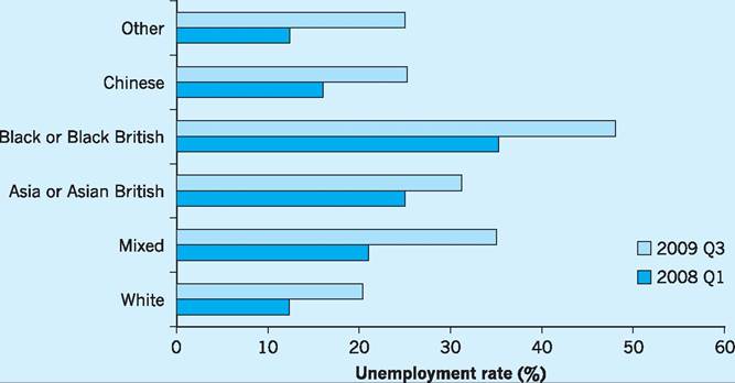
Fig. 23.3 Unemployment rates for 16-24 years of age by ethnicity. Source: ONS (various).
the population below pensionable age population belongs to one of these disadvantaged groups. A recent study (Barrett 2010) found that only 12% of people possessing none of these characteristics were economically inactive compared to 18% being economically inactive for those possessing two of these characteristics and 77% for those possessing five or six characteristics. The study showed that targeted measures in recent years had narrowed the unemployment gap between nearly all the disadvantaged groups and the population as a whole, the exception being workers with no or low qualifications. Lone parents saw the biggest narrowing of the gap and indeed were the only group to have seen an increase in their employment rate in the recent recession.
International comparisons
Unemployment rates in most countries have fallen since the mid-1980s, although not back to the low levels experienced in the 1960s. However, some countries have been less successful in reducing unemployment than others. As can be seen from Table 23.3, the big four countries in the eurozone, namely Germany, France, Italy and Spain, have had little success in reducing unemployment rates, whilst the Japanese unemployment rate has risen steadily since the early 1990s. The recent recession saw a steep rise in unemployment in all countries except for Germany and the Netherlands.
Table 23.3 Comparative unemployment rates (%) (standardized).
| 1965-72 | 1973-79 | 1980-87 | 1988-92 | 1993-02 | 2008 | 20102 | |
| France | 2.3 | 4.3 | 8.9 | 9.3 | 10.7 | 7.4 | 10.0 |
| Germany1 | 0.8 | 2.9 | 6.1 | 5.5 | 8.5 | 7.5 | 6.9 |
| Italy | 4.2 | 4.5 | 6.7 | 9.1 | 10.7 | 6.7 | 8.4 |
| Japan | 1.3 | 1.8 | 2.5 | 2.2 | 3.9 | 4.0 | 5.2 |
| Netherlands | 1.7 | 4.7 | 10.0 | 6.1 | 4.6 | 3.9 | 4.4 |
| Spain | 2.7 | 4.9 | 17.6 | 17.4 | 18.4 | 11.3 | 20.3 |
| Sweden | 1.6 | 1.6 | 2.3 | 2.7 | 7.8 | 6.2 | 8.5 |
| UK | 3.1 | 4.8 | 10.5 | 8.2 | 7.0 | bgcolor=white>5.87.8 | |
| US | 4.3 | 6.4 | 7.6 | 6.1 | 5.2 | 7.9 | 9.6 |
1West Germany up to 1992; the whole of Germany from 1993. 2July.
Sources: Adapted from OECD Economic Outlook (various); Eurostat.
Unemployment and economic theory
The traditional way of analysing the unemployment problem has been to try and identify the various types of unemployment by cause, this being seen as the first step towards formulating appropriate policy. Economists often distinguish between frictional, structural, classical and demand-deficiency (Keynesian) unemployment. Some would argue that a further type of unemployment should be distinguished, namely technological unemployment. We now consider each ‘type’ in more detail.
Frictional unemployment
Frictional unemployment results from the time it takes workers to move between jobs. It is a consequence of short-run changes in the labour market that constantly occur in a dynamic economy. Workers who leave their jobs to search for better ones require time because of the imperfections in the labour market. For example, workers are never fully aware of all the possible jobs, wages and other elements in the remuneration package, so that the first job a worker is offered is unlikely to be the one for which he or she is best suited. It is rational, therefore, for workers to spend time familiarizing themselves with the job market even though there will be costs involved in this search, namely lost earnings, postage, telephone calls, internet searches etc. These ‘search’ costs can, however, be seen from the workers’ point of view as an investment, the gain being higher future income. In principle, the economy should also gain from this search behaviour, through higher productivity as workers find jobs that are more appropriate to their skills.
Any measures that reduce the search time will reduce the amount of frictional unemployment.
Improving the transmission of job information, permitting workers to acquire knowledge of the labour market more quickly, is one such measure. A more controversial issue is how the level of unemployment benefit affects search time. It could be argued that by reducing the workers’ cost of searching, increased unemployment benefit will lead to more search activity and a higher level of frictional unemployment. On the other hand, a reduction in unemployment benefit, though perhaps leading (via less search) to lower frictional unemployment, could also lead to a less efficient allocation of resources, with workers having to take the first job that comes along regardless of how appropriate it was to their skills.
Structural unemployment
Structural unemployment arises from longer-term changes in the structure of the economy, resulting in changes in the demand for, and supply of, labour in specific industries, regions and occupations. It could be caused by changes in the comparative cost position of an industry or a region, by technological progress or by changes in the pattern of final demand. Examples of structural unemployment are not difficult to find for the UK economy and might include shipbuilding, textile, steel and motor-vehicle workers, i.e. workers in manufacturing industries where the UK has largely lost its comparative advantage over other countries (e.g. newly industrialized countries). On the other hand, the emerging unemployment in the printing industry and in clerical occupations has more to do with technological progress, which enables information to be processed, stored and retrieved more quickly, so that fewer people are required per unit of output (see below). Yet again, structural unemployment may be due to a shift in demand away from an established product, as with the decline of the coal industry following the move to gas-fired power stations.
The structurally unemployed are therefore people who are available for work, but whose skills and locations do not match those of unfilled vacancies. Structural unemployment is likely to reach high levels if the rate of decline for a country’s traditional products is rapid and if the labour market adjusts slowly to such changes. Indeed, adjustments are likely to be slow since they are costly to make. From the workers’ point of view it may require retraining in new skills and relocation, whilst from the firms’ point of view it often means abandoning their familiar products and processes and investing in new and often untried ones. This process of adjustment is, of course, easier the more buoyant the economy.
At a broader level, one of the most important issues facing developed countries is whether they will be able to generate enough output to finance the necessary increase in service occupations required to absorb those released by the manufacturing sector. Whilst manufacturing accounted for 30.1% of employment in the EU in 1970, it accounted for only around 22% in 2006, and most forecasts see this structural trend continuing (see Chapter 1). In the UK employment in manufacturing fell from 24.7% of the workforce in 1978 to 8.2% in 2010. The way in which the developed world manages this structural transition over the medium term will be one of the key determinants of future levels of employment.
Technological unemployment
New technologies have substantially raised output per unit of labour input (labour productivity) and per unit of factor input, both labour and capital (total factor productivity). There has been much concern that the impact of these productivity gains has been to reduce jobs, i.e. to create technological unemployment. We now consider the principles which will in fact determine whether or not jobs will be lost (or gained) as a result of technological change.
Higher output per unit of factor input reduces costs of production, provided only that wage rates and other factor price increases do not absorb the whole of the productivity gain. Computer-controlled machine tools are a case in point. Data from Renault show that the use of DNC machine tools resulted in machining costs one-third less than those of generalpurpose machine tools at the same level of output. Lower costs will cause the profit-maximizing firm to lower price and raise output under most market forms, as in Fig. 23.4. A downward shift of the average cost curve, via the new technologies, lowers the marginal cost curve from MC1 to MC2. The profitmaximizing price/output combination (MC = MR) now changes from P1/Q1 to P2/Q2. Price has fallen, output has risen.
The dual effect on employment of higher output per unit of labour (and capital) input can usefully be illustrated from Fig. 23.4. The curve Q = F(N) is the familiar production function of economic theory, showing how output (Q) varies with labour input (N), with capital and other factors assumed constant. On the one hand, the higher labour productivity from technical change shifts the production function outwards to the dashed line Q' = F(N). The original output Q1 can now be produced with less labour, i.e. with only N2 labour input instead of N1 as previously. On the other hand, the cost and price reduction has so raised demand that more output is required. We now move along the new production function Q' until we reach Q2 output, which requires N3 labour input. In our example, the reduction in labour required per unit output has been more than compensated for by the expansion of output, via lower price. Employment has, in fact, risen from N1 to N3.
This analysis highlights a number of points on which the final employment outcome for a firm adopting the new techniques will depend.
1 The relationship between new technology and labour productivity, i.e. the extent to which the production function Q shifts outwards.
2 The relationship between labour productivity and cost, i.e. the extent to which the marginal cost curve shifts downwards.
3 The relationship between cost and price, i.e. the extent to which cost reductions are passed on to consumers as lower prices.
4 The relationship between lower price and higher demand, i.e. the price elasticity of the demand curve.
Suppose, for instance, that the new process halved labour input per unit output. If this increase in labour productivity (1 above) reduces cost (2 above) and price (3 above), and output doubled (4 above), then the same total labour input would be required. If output more than doubled, then more labour would be employed. The magnitude of the four relationships above will determine whether the firm offers the same, more or less employment after technical change in the production process.
Although a more detailed treatment must be sought elsewhere, there is in fact a fifth relationship crucial to the final employment outcome, namely, the extent to which any higher total factor productivity arising from a technological innovation can be separately attributed to capital or to labour. An innovation is said to be capital saving when the marginal product of capital rises relative to that of labour, and
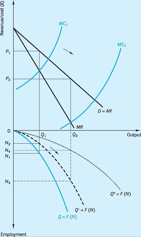
Fig. 23.4 Technical change and the level of employment.
labour saving when the converse applies. This whole issue is surrounded by problems of concept and measurement. We can, however, use Fig. 23.4 to present the outline of the argument.
Suppose we take the dashed line Q' = F(N) to represent a situation in which the new technology is capital saving (with only a small rise in labour productivity), so that the new and higher output Q2 requires considerable extra labour to produce it (N3 employment). If, on the other hand, the new technology were labour saving (with a substantial rise in labour productivity), then the new dotted line Q" = F(N) in Fig. 23.4 would be more appropriate. Output Q2 would now only require employment N4. The prospects for higher employment would therefore appear more favourable when innovations are capital saving, raising the marginal product of capital relative to that of labour.
Broadly speaking, the scenario most favourable to employment would be where a small increase in (labour) productivity significantly reduces both cost and price, leading to a substantial rise in demand.
Classical unemployment
Unemployment may be associated, in the classical view, with real wages that are ‘too high’. In this case, trade unions have used their power to force the real wage above the market clearing level or have prevented it from falling to the market clearing level after a change in the supply or demand conditions. A government minimum wage above the equilibrium wage could also generate such classical unemployment. In the 1970s there was a revival in this line of thought. The monetarist and new classical economists argued that whilst, for the most part, the economy would be at ‘full employment’, there might be times when firms and workers would overestimate the rate of inflation. If firms pay money wage increases based on such false price expectations, this will lead to (temporarily) higher real wages and reduced employment. Figure 23.5 illustrates classical unemployment using the familiar labour market diagram.
The labour demand curve has a negative slope to reflect the usual assumption that the demand for
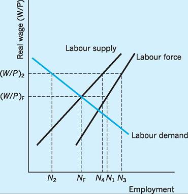
Fig. 23.5 ‘Voluntary' or equilibrium unemployment and the real wage.
labour rises as the real wage falls. The labour force curve has a positive slope to reflect increased labour force participation as real wages rise. The labour supply curve represents those willing and able to take jobs at a given real wage. The market clearing real wage is (W7P)f, giving employment equal to the full employment level Nf and unemployment equal to N1 - Nf. This equilibrium level of unemployment is considered to be entirely voluntary. However, if the real wage (W∕P)2 is above the market clearing level ( W7P)f for whatever reason, then employment falls to N2 and unemployment increases to N3 - N2 of which the portion N3 - N4 could be regarded as ‘voluntary’. In the classical view the remaining ‘involuntary’ unemployment N4 - N2 could not persist for long. The unemployed would exert downward pressure on money wages, and the real wage would fall back to the market clearing level.
Demand-deficient unemployment
Keynes criticized the view that unemployment is caused by too high real wages. He considered that the cause of mass unemployment in the 1930s was not to be found in the market for labour, but was rather a result of too little demand in the market for goods. This lack of overall demand together with an assumed downward stickiness in wages and prices leaves the economy trapped for long periods with high levels of unemployment. The downward stickiness in wages (and therefore prices) thwarts the operation of the real balance effect, whereby lower prices raise real incomes and thereby increase consumer spending.1 Since no automatic tendency exists to return the economy to full employment by generating sufficient aggregate demand in the goods market, Keynesians would advocate some form of expansionary government demand-management policy. Demand-deficient (Keynesian) unemployment is illustrated in Fig. 23.6.
Aggregate demand (AD) determines the level of output Y2 (assume Yf is full employment output - i.e. only ‘voluntary’ unemployment). Given this level of output and the production function in the economy, firms will need to employ only N2 workers to meet the demand for their product. The effective demand for labour is traced out by the points a-b-N2. Note that the real wage could be anywhere between (W7P)2 and (W7P)3. A cut in real wages would not restore employment to its full employment level (Nf) if
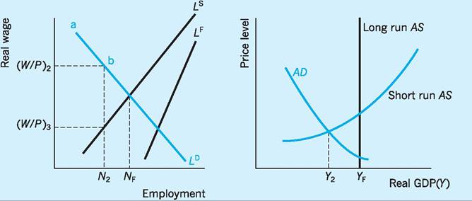
Fig. 23.6 Demand-deficient unemployment.
aggregate demand for output remains unchanged at a level consistent with output Y2.
A framework for thinking about unemployment
above the structural level in all the countries in our sample, apart from Germany. The argument would now be that demand needs to increase to encourage firms to hire the unemployed workers. The key issue is whether this extra demand should come from public sector expenditure or whether the private sector is capable or indeed willing to provide it.
One useful way of thinking about unemployment, which is especially helpful from a policy perspective, is to distinguish between ‘cyclical unemployment’ which results from a deficiency of aggregate demand (e.g. during the downswing of the business cycle) and ‘sustainable unemployment’. Sustainable unemployment is the level below which tightness in the labour market will lead to an increasing rate of wage and price inflation. The sustainable level of unemployment is variously referred to as the ‘natural rate of unemployment’ (NRU), the ‘non-accelerating inflation rate of unemployment’ (NAIRU) or, as in OECD publications, the ‘structural’ rate of unemployment.
At any moment in time therefore:

Figure 23.7 illustrates these two components for several OECD (advanced industrialized) countries in 2010. In 2006, prior to the recent recession, some countries (Ireland, the UK, Italy, Spain) had unemployment rates below the structural (sustainable) rate. The implication is that demand was too high and that future inflation was a danger. As Fig. 23.7 shows, the recession has had the effect of pushing unemployment
The natural rate of unemployment (NRU) and the NAIRU
Given the central role of these concepts in discussions of unemployment, it might be useful to consider the NRU and NAIRU in rather more detail.
Natural rate of unemployment (NRU)
The NRU was introduced into economics by Milton Friedman (Friedman 1968). It can be thought of as being derived from a competitive labour market with flexible real wages, with the natural rate of unemployment being determined by the equilibrium of labour supply and demand. The usual labour market diagram of Fig. 23.8 can be used to illustrate this. Here labour demand, Ld, reflects the marginal revenue product of workers, i.e. the extra revenue contributed by employing the last worker. This is downward sloping in line with the assumption of a diminishing marginal physical product for workers (see Chapter 14). Labour supply, Ls, represents all those workers willing and able (i.e. they have the right skills and are in the right location) to accept jobs at a given real wage. The labour force, Lf, shows the total number
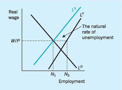
Fig. 23.8 Finding the natural rate of unemployment (NRU).
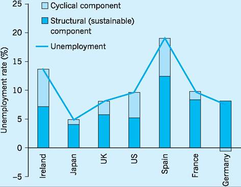
Fig. 23.7 Unemployment rate, structural (sustainable) and cyclical components, 2010. Source: OECD (various).
of workers who consider themselves to be members of the labour force at any given real wage; of course not all of these are willing or able to accept job offers, perhaps because they are still searching for a better offer or because they have not yet acquired the appropriate skills or are not in an appropriate location. Note the convergence of Ls and Lf as the real wage rises. This reflects the reduction in the ‘replacement ratio’ (i.e. ratio of benefits when out of work to earnings when in work) when real wages rise, given the current level of unemployment benefits. Such a reduction in the ‘replacement ratio’ could be expected to result in a higher proportion of the labour force being willing and able to accept jobs as the real wage rate rises (see Chapter 14).
At the equilibrium real wage (W/P) in Fig. 23.8, N1 workers are willing and able to accept job offers whereas N2 workers consider themselves to be members of the labour force. That part of the labour force unwilling or unable to accept job offers at the equilibrium real wage (N2 - N1) is defined as being the natural rate of unemployment (NRU). In terms of our earlier classification of the unemployed, the NRU can be regarded as including both the frictionally and structurally unemployed.
It can be seen that anything that reduces the labour supply (the numbers willing and able to accept a job at a given real wage) will, other things being equal, cause the NRU to increase. Possible factors might include an increase in the level or availability of unemployment benefits, thereby encouraging unemployed members of the labour force to engage in more prolonged search activity. An increase in trade union power might also reduce the numbers willing and able to accept a job at a given real wage, especially if the trade union is able to restrict the effective labour supply as part of a strategy for raising wages. A reduced labour supply might also result from increased technological change or increased global competition, both of which change the nature of the labour market skills required for employment. Higher taxes on earned income are also likely to reduce the labour supply at any given real wage.
Similarly anything that reduces the labour demand will, other things being equal, cause the NRU to increase. A fall in the marginal revenue product of labour, via a fall in marginal physical productivity or in the product price, might be expected to reduce labour demand. Many economists believe that the two sharp oil price increases in the 1970s had this effect, with the resulting fall in aggregate demand causing firms to cut back on capital spending, reducing the overall capital stock and hence the marginal physical productivity of labour.
Non-accelerating inflation rate of unemployment (NAIRU)
Unlike the NRU which assumes a competitive labour market, the NAIRU is usually developed from a model that recognizes imperfect competition in the labour market (Layard 1986). The ‘sustainable’ level of unemployment (i.e. the level consistent with the inflation rate being unchanged) is seen here as being the result of a bargaining equilibrium between firms and workers rather than a market clearing outcome. The two sides of the labour market are seen as engaged in a constant struggle over the available real output per head. If the claims of the two sides are inconsistent, in that they add up to more than the real output per head available, then each side will try to safeguard its own claim by using its market power. Workers will claim higher money wages and firms will raise their product prices. The result of such a power struggle will then be rising inflation.
Figure 23.9 illustrates the determination of the NAIRU. At any particular moment there is a limit to the real wage the economy can provide, given labour productivity and the mark-up that firms typically apply to costs. This limit is the feasible real wage (WIP}*. At the same time, the target real wage reflects the aspirations of workers. It seems likely that this target will be influenced by the level of demand in the economy, as reflected by the unemployment rate. When demand is high and unemployment is low, workers will feel more able to negotiate wage increases than when demand is low and unemployment high. There will be some level of unemployment where workers’ aspirations are equal to the real wage
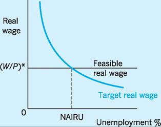
Fig. 23.9 The determination of the NAIRU.
that firms are willing to offer; this is the NAIRU. In other words, NAIRU is determined by the intersection of the target and feasible real wage curves in Fig. 23.9. If unemployment were pushed below the NAIRU by government expansionary policy, then workers would seek a real wage above the feasible level; in an attempt to secure this they would demand higher money wages. If they were successful in securing these, firms would maintain their mark-up over costs by raising prices. If unemployment were to remain below the NAIRU, then a wage-price spiral would ensue. At some stage the government would have to allow unemployment to rise towards the NAIRU to end the rising inflation rate.
To sum up, then, the NAIRU is seen as being the level of unemployment necessary to keep inflation from rising. Anything which shifts the target or feasible real wage curves in Fig. 23.9 will affect the NAIRU.
Any factor that enables or encourages workers to increase the target real wage for a given level of unemployment will clearly increase the NAIRU, shifting the target real wage curve upwards and to the right. Such factors might include any or all of the following:
■ an increase in benefits and their duration;
■ an increase in trade union power or greater employment protection (both reducing the fear of unemployment);
■ increased structural unemployment (the unemployed now compete less effectively with the employed because they have the wrong skills or are in the wrong place);
■ an increase in the long-term unemployed as a proportion of total unemployment (the longterm unemployed compete less effectively with the employed for jobs);
■ an increase in taxes on earnings which reduces the post-tax real wage and leads workers to seek a higher pre-tax real wage.
Similarly any factor that reduces the feasible real wage will increase the NAIRU. Such factors might include any or all of the following:
■ reduced labour productivity;
■ unfavourable movements in the Terms of Trade (i.e. a fall in the ratio of export to import prices), reducing the share of output going to domestic employees and raising that going to foreign employees;
■ higher dividends reducing the share of output going to employees and raising that going to shareholders;
■ more ‘leapfrogging’ by which one group of workers use a pay increase by others to justify their own higher pay demands.
The idea that the best policy-makers can do in the short run is to keep demand at a level such that unemployment is at or near the NAIRU, whilst in the long run reforming labour market incentives and institutions to lower the NAIRU, has dominated economic policy making for the last 30 years. However, this strategy is, of course, not without its critics, not least because of considerable variability in the estimates of the NAIRU that have been made for the UK over various time periods, indicated in Table 23.4. Galbraith (1997) argued that it was time to abandon the NAIRU on theoretical grounds and also because attempts to keep its level down had become a ‘professional embarrassment’. In addition, policy-makers, arguably too much concerned with inflation, had run the economy with too low a level of demand and too high a level of unemployment, causing the NAIRU to increase (see p. 492 on Hysteresis). Storm and Naastepad (2009) similarly argue that adherence to the NAIRU as a guide to policy in France, Germany and Italy (as compared to US policy) has led to between 900,000 and 2.4 million extra European workers being (unnecessarily) unemployed. They argue that more expansionary policies, aimed at full employment, and higher labour productivity growth policies followed by the Nordic countries have provided better outcomes compared to a rigid following the NAIRU framework.
I Unemployment in the OECD
Two important puzzles face applied economists when considering data on unemployment in the advanced industrialized countries of the OECD. One puzzle involves explaining why unemployment has been much higher in almost all OECD countries during the 1980s and 1990s than it had been in the decades following the Second World War. The second puzzle involves explaining why such large variations have been recorded in unemployment rates between the OECD countries.
A study of cross-country differences in unemployment rates (Nickell 1998) attempted to assess the impact on unemployment of a variety of factors. For example, Nickell estimated that a 10% increase in the ‘replacement ratio’ and a one-year increase in the duration of entitlement to unemployment benefits would result in a 25% increase in unemployment, while a 10% increase in trade union density would result in a 60% increase in unemployment. On the other hand, a 5% reduction in the overall tax rate would reduce unemployment by 15% and a 2% cut in the real interest rate (a substantial cut) would reduce unemployment by around 10%. He found that policies involving an increase in labour market ‘rigidity’ (such as improved labour standards and greater employment protection) had little impact on overall unemployment. Nickell argued that such variables, despite problems of definition and measurement across countries, do shed some light on why unemployment varies a great deal between countries. For example, Spain, with its high replacement ratios, long benefit duration, rather high tax rates on earnings and relatively ‘rigid’ labour market, suffers from high unemployment, as might be expected from Nickell’s analysis, whereas the US, with its relatively low replacement ratios, short benefit duration, low tax rates on earnings, flexible labour market and low union coverage, has relatively low unemployment.
Table 23.4 Estimates of the UK NAIRU.
| Time period 1966-73 1974-80 | 1981-87 | 1989-90 | 1996-99 | 2002 2007 |
| NAIRU range 1.6-5.6% 4.5-7.3% | 5.2-9.9% | 3.5-8.1% | 6% approx. | 5.25% approx. 5.3% |
| Sources: OECD Economics Department Working Papers 649 (Gianella et al. 2008); Bank of England Quarterly Bulletin (1993), Vol. 33, No. 2; Bank of England (1998) Inflation Report, August; HM Treasury (2002b) Trend Growth; Recent | ||||
| Developments and Prospects, April. | ||||
Nickell goes on to argue that although his variables usefully explain cross-country comparisons, they are less useful in explaining the time-series pattern of OECD unemployment (see also Bean 1994). For example, when comparing the higher unemployment of the 1990s with the much lower unemployment of the 1960s, Nickell was surprised to find that today’s replacement ratios are no more generous, trade union militancy no worse, real interest rates not much higher, and labour markets not much more rigid than all of these factors had been in the 1960s and yet unemployment is so much higher.
Concentrating on the UK alone, rather than on cross-country comparisons, Nickell (1998) estimated that the fourfold rise in the numbers unemployed since the 1960s could comfortably be explained by a model including the replacement ratio, the Terms of Trade, skills mismatch, union pressure, industrial turbulence, the tax ‘wedge’ and the real interest rate. The variables making the most important (percentage) contributions in explaining the overall rise in unemployment have been skills mismatch 14%, union pressure 19% and tax ‘wedge’ 23%, but the real interest rate only 3.5%.
A rather different view was offered by Phelps and Zoega (1998) who suggested that two global forces, namely sharp rises in oil prices in the 1970s and in real world interest rates in the 1980s and early 1990s, have been the major factors responsible for the observed increases in worldwide unemployment since the 1960s.
Higher oil prices reduce labour productivity by reducing the proportion of the existing capital stock which can be regarded as ‘economically efficient’; for example, oil-intensive capital equipment becomes effectively redundant. As well as diminishing the ‘economically efficient’ capital stock, and with it labour productivity, higher oil prices are seen by Phelps and Zoega as contributing to higher unemployment by diminishing net exports (exports minus imports) for many OECD countries. The non-oil exporting OECD countries have been particularly hard-hit by ever increasing import bills for oil and ‘oil-based’ products.
The Phelps and Zoega model sees hiring rates for workers as heavily dependent on both net productivity and the real interest rate. As well as the slowdown in productivity growth experienced in most countries following oil-price shocks, the steep rises in global real interest rates also experienced at such times further reduce the hiring rate for labour, resulting in substantial increases in levels of unemployment. Higher real interest rates particularly discourage the hiring of workers who require a substantial investment in human capital, such as the large numbers of higher skilled and well-educated workers required by many high-technology, ‘information age’ industries.
Unemployment persistence and hysteresis
In the mid-1980s oil prices fell, trade union power diminished compared to the 1970s, the replacement ratio fell, and yet unemployment kept on rising, at least in Europe. One explanation might be that demand-deficient unemployment had risen because governments were trying to control inflation by running the economy with unemployment above the NAIRU. However, inflation did not fall in the mid- 1980s, leading some economists to the view that a period of high unemployment resulting from contractionary demand management might lead to the NAIRU itself increasing. The idea that there might be a mechanism whereby a rise in unemployment increases the equilibrium (or natural) rate of unemployment is known as hysteresis. There are several possible mechanisms to explain hysteresis in European unemployment.
One explanation of hysteresis involves the insideroutsider hypothesis (Blanchard and Summers 1986; Lindbeck and Snower 1988). Insiders are the unionized employed who pay little attention to the interests of the unemployed outsiders. For a variety of reasons (such as turnover costs, firm-specific human capital and the possibility of refusing to co-operate with newly hired outsiders), insiders do not fear that they will be replaced by outsiders. Of course in practice, if the demand for labour falls, then some insiders may lose their jobs and become outsiders. Once labour demand recovers, however, the smaller pool of insiders who remain will exploit their relative scarcity by negotiating higher wages for themselves rather than accepting wage moderation and allowing the employment of more outsiders. The economy therefore settles at a higher-wage, lower-employment equilibrium.
A second explanation of hysteresis concentrates on the role of the long-term unemployed; in other words this approach concentrates on the role of the outsiders rather than on the wage-determining role of the insiders. The long-term unemployed are seen as effectively having withdrawn from the labour force (they search less effectively, they lose their skills and employers see them as a bad risk). The result is that they do not exert much downward pressure on wage setting, so that a higher level of unemployment is required to exert the same control on inflation when the long-term unemployed increase as a proportion of the total unemployed. Empirical evidence certainly suggests that when European unemployment persists the effect is to increase the proportion of the longterm unemployed in total unemployment, so that the equilibrium (or natural) rate of unemployment rises.
A third explanation of hysteresis involves the effect of recessions on the capital stock. As aggregate demand falls, firms go out of business and investment plans are shelved, reducing the capital-to-labour ratio and therefore the marginal productivity of labour (shifting the labour demand curve to the left). From the point of view of the NAIRU model there has been a reduction in the ‘feasible real wage’. Whichever way we look at it, the equilibrium (or natural) rate of unemployment rises.
A fourth explanation of hysteresis involves the suggestion that a more highly regulated labour market discourages recruitment, and may lead to higher equilibrium unemployment after a downturn in demand (see Bean 1994).
What can be done to reduce unemployment?
In 1994, at a time of high and persistent unemployment, the OECD published its Jobs Study (OECD 1994). This study, together with the OECD’s Jobs Strategy (1998), made more than 60 policy recommendations and provided a blueprint aimed at creating jobs and reducing unemployment, whilst at the same time maintaining social cohesion. As Coats (2006) points out in Who’s Afraid of Labour Market Flexibility?, the strategy was a mixture of Keynesian demand management (deficit spending in recessions and fiscal consolidation in booms), growth theory (with its emphasis on entrepreneurship, research and development) and labour market flexibility (with its emphasis on job skills). The key recommendations were as follows.
■ Set macroeconomic policy to encourage non- inflationary growth.
■ Enhance the creation and diffusion of technology.
■ Increase working time flexibility.
■ Encourage entrepreneurship and eliminate restrictions on the creation and expansion of enterprises.
■ Make wage and labour costs flexible and responsive to local conditions and skill levels, particularly for young workers.
■ Reform employment security provisions that inhibit recruitment.
■ Strengthen the emphasis on ‘active’ labour market policies.
■ Improve the education and skills of the labour force.
■ Reform ‘unemployment and related’ benefits and the tax system to improve the functioning of the job market, whilst not jeopardizing society’s equity goals.
■ Enhance product market competition to reduce monopolistic tendencies and weaken insideroutsider mechanisms, thereby leading to a more dynamic economy.
In June 2006 a revised study was published (OECD 2006) reviewing the progress that had been made in improving the labour markets since 1994. Its conclusions were that some progress has been made in most but not all countries. At the same time the challenges and dangers have become broader and include a more rapid pace of technological advance, globalization with the associated increase in competition from the extra labour force in China and India, and the demographic problem of an ageing workforce in many countries.
Over the 12 years the OECD noted that the trend rise in unemployment had been reversed or at least stabilized. In some countries, notably Finland, Spain and Ireland, there had been substantial reductions (9.3, 11.2 and 10.0 percentage points respectively between 1994 and 2006). Other countries that adopted many, if not all, of the Job Strategy recommendations had also done well. The UK, for example, reduced unemployment over the same period by 4.1 percentage points. However, it was also the case that other countries that had adopted the Nordic ‘flexicurity’ approach such as Denmark with its easy hire-and-fire but strong support for the unemployed (who receive 65% of work income compared with only 18% in the UK), Austria and the Netherlands, all of which had similar approaches, had also done relatively well. Other countries that the OECD regarded as not having reformed their labour markets sufficiently, such as Germany, France and Italy, had done less well despite strong global growth over that period.
Active labour market policies
The last decade has seen an emphasis on ‘activating’ the unemployed and other benefit recipients. The various OECD countries have differed in their specific implementation of this strategy, but most have used a ‘carrot and stick approach’. High-quality employment services and strong job search incentives have been reinforced by the threat of benefit reduction or removal. The OECD argued that if properly designed, such ‘active labour market policies’ (ALPs) have led to improved labour market outcomes. The UK has gone further down the road of these ALPs than have most other OECD countries. The last Labour government set up the various New Deal programmes and later the ‘Pathways to Work’ programme for people with disabilities in an attempt to increase the employment of the various groups. The introduction of the minimum wage and reforms of tax and benefits were also policies directed towards increasing the incentives to move into work (see Chapter 19). At the same time, it has also been argued that UK benefit recipients face some of the toughest hurdles in order to receive or continue receiving benefits (Daguerre and Etherington, 2009). It is difficult to assess the effectiveness of these programmes, but Daguerre and Etherington argue that there have been mixed results and that it is important to tailor ALPs to the most needy and to ensure early and high quality interventions and individualised assistance as it is clear that ‘one size’ does not fit all.
I The great recession
The ‘great recession’ can be dated from late 2007 for the US and early 2008 for many other countries and regions, including the UK and Europe. The ILO has estimated that this recession has resulted in an extra 34 million unemployed people worldwide, with unemployment in the OECD countries reaching a post-war high of 8.7% in March 2010. Particularly badly affected have been young workers, with youth unemployment in the OECD rising by 7%, nearly four times the rate for other employees.
It is interesting to note that not all countries have had the same experience; in fact, the disparity of experience seems to have been greater than in previous recessions! As Fig. 23.10 shows, the US and Spain have shed the largest numbers of workers relative to the fall in GDP, the suggestion being that workers in the US have a fairly low level of job protection and so are more easily released. Spain suffered job losses partly as a result of the collapse of the labourintensive housing market bubble (Ireland also), but also because a large proportion of its workers, especially the young, immigrants and the unskilled, are on short-term (temporary) contracts with very little job protection. Stronger employment protection measures, in the view of many analysts, maintained employment in Germany and France, as did short-term and more flexible working arrangements (e.g. a reduction in weekly hours worked) in Germany, some other European countries and Japan, which helped dampen the effects of the recession on unemployment. Labour hoarding of this type is, however, not without its
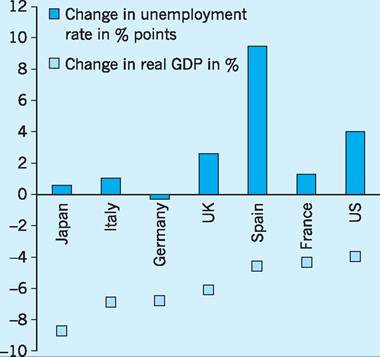
Fig. 23.10 Change in unemployment and GDP from peak to trough: selected OECD countries.
Source: OECD Economic Outlook (various).
costs, as it results in lower labour productivity and may lead to the danger of a jobless recovery. The OECD (2010) has estimated, for example, that output in Japan could rise by as much as 7% during the recovery without firms needing to hire any new workers, if hours per worker and productivity levels return to the pre-crisis level. Keeping workers engaged in the labour market nevertheless has many overall benefits and lowers the danger of hysteresis (see p. 492).
In the UK, GDP fell by 8% in the two years to Q1 2010, a much larger fall than in the previous two recessions at the start of the 1980s and 1990s. Employment, however, has fallen by much less than in those recessions, i.e. by 1.9% as against the 2.4% in the 1980s recession and the 3.4% in the 1990s recession. A further difference is also worth noting, namely that real wages per hour rose less rapidly in the current recession as compared to the previous recessions, putting less pressure on firms to shed labour. Hours worked per worker fell as in previous recessions but by a similar amount.
Faccini and Hackworth (2010) have examined the reasons that have helped dampen the fall in employment. First, they conclude that some of the explanation can be found in the changes in the economy which have occurred since the 1990s. The 1990s recession was preceded by rapid price and wage inflation, and subsequently prices fell more rapidly than money wages, with output prices changing on average each four months whereas wages only changed on average annually! As a result, real wages rose, forcing firms to reduce employment. The current recession was, however, preceded by low and stable inflation so there was less need for downward price adjustments and hence real wages may have risen less rapidly than before, putting less pressure on firms to cut employment.
A second explanation might be found in structural changes in the labour market which have meant that firms are more willing, at least in the short term, to accept lower productivity and workers are more willing to accept lower real wages. Increased hiring and firing cost are seen as a reason for such responses by employers and weaker unionization. Lower unionization since the 1990s (see Chapter 14) may explain some of the differences from the earlier recessions, although most of the decline in unionization occurred before the current recession.
Other factors which might explain these differences between respective recessions might include more pessimistic expectations of employees, leading to increased concerns about future jobs and hence greater wage moderation. Labour supply also impacts on wages, and the labour force participation rate seems to have held up better than in previous recessions. Older workers may be more concerned about future pensions, given the financial crisis and the removal of many final salary pensions, and households in general may be more concerned about future incomes, leading both groups to work longer, whether in years before retirement or before withdrawing from the labour force, respectively. The 25% reduction in the effective sterling exchange rate between mid-2007 and early 2009 might also have had an influence in the UK; the higher import prices helping UK-based firms to compete against more expensive imports, which may have helped reduce the need for cost savings via cutting jobs. Lower sterling export prices may also have reduced the need for UK-based exporters to reduce employment.
Overall, the unusual behaviour of the UK labour market in the recent recession is likely to be partly due to an increased flexibility in real wages relative to employment and partly due to other factors such as the supply of labour and the exchange rate depreciation.
I Conclusion
Unemployment is determined by the level of demand in the economy. If demand is too low, then unemployment will be above the equilibrium rate (structural rate or NAIRU); if demand is too high, then unemployment will be below the NAIRU and, in the absence of other offsetting factors, the inflation rate will begin to rise. The implication for policy is that demand management should aim to keep unemployment as close to the NAIRU as possible, whilst labour and goods market initiatives should aim to reduce the NAIRU.
As the OECD has pointed out, the immediate need is to use fiscal and monetary policy to reduce unemployment back to its structural level (NAIRU) by eliminating cyclical unemployment and preventing the NAIRU rising as a result of the current crisis (the hysteresis effect). A continuation of the structural reforms outlined earlier together with effective expenditure on active labour policies (ALP) and an emphasis on the most vulnerable groups are all necessary if we are to ensure a sustained job-rich recovery.
Key points
■ Successive ‘unemployment cycles’ (peak to peak) have tended to result in higher unemployment rates.
■ The ILO (survey) method of measuring the unemployed differs from the claimant (administrative record) method used in the UK.
■ Unemployment in the UK can be disaggregated into regional, occupational, gender, age, ethnically-based and qualification-related unemployment.
■ The major types of unemployment include frictional (temporary), structural (changing patterns of demand), technological (changing technology), classical (‘excessive’ real wages) and demand-deficient (inadequate demand) categories.
■ The natural rate of unemployment (NRU) is the voluntary unemployment (labour force - labour supply) existing at the real wage level which ‘clears’ the markets.
■ The non-accelerating inflation rate of unemployment (NAIRU) is that level of unemployment which equates the feasible real wage with the target real wage. It is the unemployment rate at which inflation is constant.
■ Progress has been made in reducing the UK NAIRU since the 1980s.
■ Combinations of policies are required to combat unemployment.
Now try the self-check questions for this chapter on the Companion Website. You will also find useful links to relevant websites.
Note
1 The downward stickiness in wages (wage rigidity) and therefore prices also thwarts the interest rate and foreign trade effects which might stimulate recovery. In the ‘interest rate effect’, lower prices mean an increase in real money supply, lowering the ‘price’ of money (interest rates) and thereby raising the investment component of aggregate demand. In the ‘foreign trade effect’, lower prices mean more competitive exports and more competitive (home-produced) substitutes for imports, a rise in exports and a fall in imports again stimulating (net) aggregate demand.
References and further reading
Bank of England (1998) Inflation Report, August, London.
Bank of England Quarterly Bulletin (1993) Volume 33, no. 2.
Barrett, R. (2010) Disadvantaged groups in the labour market, Economic and Labour Market Review, 4 (6): 18-24.
Barro, R. J. (1998) Macroeconomics, Cambridge MA, MIT Press.
Barwell, R. (2000) Age structure and the UK unemployment rate, Bank of England Quarterly Bulletin, 40(3), August.
Bean, C. (1994) European unemployment: a survey, Journal of Economic Literature, 32, June.
Begg, D., Fischer, S. and Dornbusch, R. (1994) Economics, London, McGraw-Hill. Benassy-Quere, A. and Coeure, B. (2010) Economic Policy, Oxford, Oxford University Press.
Berthoud, R. (2003) Multiple Disadvantage in Employment: A Quantitative Analysis, Institute for Social and Economic Research, Colchester, University of Essex.
Blanchard, D. and Summers, L. (1986) Hysteresis and the European unemployment problem, NBER Macroeconomic Annual, Cambridge, MA, National Bureau of Economic Research. Clark, A. and Layard, R. (1989) UK Unemployment, Oxford, Heinemann Educational.
Coats, D. (2006) Who’s Afraid of Labour Market Flexibility? London, The Work Foundation.
Daguerre, A. and Etherington, D. (2009) Active Labour Market Polices in International Context: What Works Best? Lessons for the UK, Department for Works and Pension, Working Paper 59, London, The Stationery Office. Dawson, G. (1992) Inflation and Unemployment: Causes, Consequences and Cures, Cheltenham, Edward Elgar.
Faccini, R. and Hackworth, C. (2010) Changes in output, employment and wages during recessions in the UK, Bank of England Quarterly Bulletin, first quarter.
Fothergill, S. and Gudgin, G. (1982) Unequal Growth: Urban and Regional Change in the UK, London, Heinemann.
Friedman, M. (1968) The role of monetary policy, American Economic Review, 58, March.
Galbraith, J. (1997) Time to ditch the NAIRU, Journal of Economic Perspectives, 11(1), Winter.
Gianella, C., Koske, I., Rusticelli, E. and Chatal, O. (2008) What Drives the NAIRU? Evidence From a Panel of OECD Countries, OECD Economics Department Working Papers 649, Paris, Organisation for Economic Cooperation and Development.
Giavazzi, F. and Blanchard, O. (2010) Macroeconomics: A European Perspective, Harlow, Financial Times/Prentice Hall.
HM Treasury (1998) Stability and Investment for the Long Term: Economic and Fiscal Strategy Report, London.
HM Treasury (2002a) UK Employment Action Plan, London.
HM Treasury (2002b) Trend Growth: Recent Developments and Prospects, London.
ILO-IMF (2010), The Challenges of Growth, Employment and Social Cohesion, discussion paper, Joint ILO-IMF conference in cooperation with the office of the Prime Minister of Norway, Oslo, September 13.
IPPR (2010) Youth Unemployment and the Recession, Press Release, 20 January, London, Institute for Public Policy Research.
Keynes, J. M. (1936) The General Theory of Employment, Interest and Money, Basingstoke, Macmillan.
Mishel, L. (2006) CEO Pay-to-Minimum Wage Ratio Soars, Economic Snapshot, June 26, Washington DC, Economic Policy Institute. Layard, R. (1986) How to Beat Unemployment, Oxford, Oxford University Press.
Layard, R., Nickell, S. and Jackman, R. (1994) The Unemployment Crisis, Oxford, Oxford University Press.
Lee, N. (2010) No City Left Behind? The Geography of the Recovery, London, The Work Foundation.
Lindbeck, A. and Snower, D. (1988) The InsiderOutsider Theory of Employment and Unemployment, Cambridge MA, MIT Press. Nickell, S. (1998) Unemployment: questions and some answers, Economic Journal, 108(48), May.
Nickell, S. (2003) Poverty and Worthlessness in Britain, speech given at Royal Economic Society Conference at Warwick, 8 April.
OECD (1994) Jobs Study: Facts, Analysis and Strategies, Paris, Organisation for Economic Cooperation and Development.
OECD (1998) Jobs Strategy: Progress Report, OECD Working Paper No. 196, Paris, Organisation for Economic Cooperation and Development.
OECD (2006) OECD Employment Outlook, Boosting Jobs and Income, Paris, Organisation for Economic Cooperation and Development.
OECD (2010) Return to work after the Crisis, Economic Outlook, No. 87, May, 251-92. ONS (2000) Labour Market Trends, July, London, Office for National Statistics.
Phelps, E. and Zoega, G. (1998) Natural rate theory and OECD unemployment, Economic Journal, 108(48), May.
Rowthorn, R. (1995) Capital formation and unemployment, Oxford Review of Economic Policy, 11(1), Spring.
Storm, S. and Naastepad, C. (2009) The costs of NAIRU variation, Challenge, 52(5), September- October.
More on the topic Unemployment:
- Unemployment
- First Encounter with Economics
- Introduction
- About the Book
- The First Draft, 1945
- HELP MOVING
- LMIs AND WAGE INEQUALITY: AN EMPIRICAL ASSESSMENT
- WOMEN AND WORK
- INDEX
- Stage of maturity