Inflation
In this chapter we first examine a number of methods of measuring inflation. We then consider the ‘costs' of inflation, both when it is fully anticipated, and when, as is usually the case, it is not.
A basic theoretical framework for understanding inflation is presented and is used to explain recent experience in the UK and elsewhere. The issues of inflation targeting and central bank independence are also considered.The linkages between inflation and the real economy are explored, as are the arguments for changing the emphasis on various monetary policy instruments in the attempt to control inflation and inflationary expectations.
Further related discussions on inflation can be found in Chapters 20 (Money and monetary policy), 21 (Financial institutions and markets), 23 (Unemployment) and 30 (Managing the global economy: post-‘credit crunch').
The definition and measurement of inflation
Inflation is a persistent tendency for the general level of prices to rise. In effect the rate of inflation measures the change in the purchasing power of money, i.e. how much more money you would need to have this year when faced with this year’s prices to be as well off as you were last year when faced with last year’s prices.
The UK has two main measures of inflation, the Consumer Price Index (CPI) and the Retail Price Index (RPI). The CPI is used as inflation target by the UK government, and the Monetary Policy Committee (MPC) of the Bank of England is given this inflation target and tasked with achieving it when it sets interest rates each month. The calculation of the CPI is based on EU definitions and so is useful for making international comparisons of inflation. The RPI was first published in 1947 and is probably the more familiar of the two measures, being used as the basis for tax allowances, state benefits, pensions and index- linked gilts.
However, from April 2011 the CPI has replaced the RPI as the price index used when calculating benefits, tax credits and public sector pensions, although the RPI will still be used to update index- linked gilts.The Consumer Price Index (CPI) and the Retail Price Index (RPI)
The simplest way to think about a price index is to imagine a huge ‘basket’ of goods and services that represents what the average consumer purchases; it includes such things as food, foreign holidays, car fuel, clothing, housing and so on. The content of the basket stays the same each year, but as prices change so does the cost of the basket. The CPI measures how the average price of this representative basket changes over time.
■ CPI. The CPI is calculated using around 700 separate and representative items, as it is obviously impracticable and unnecessary to monitor the price of all goods and services. The group ‘fruit’, for example, includes 15 different types of fruit whose price movements are thought to be representative of all types of fruit. These 15 fruit prices are then combined together to obtain the overall movement in the price of the group, ‘fruit’. The coverage of items in the CPI is broadly similar to that of the RPI except in its treatment of housing costs. The CPI does not include council tax, mortgage interest payments, house depreciation, buildings insurance and one or two other housing costs. On the other hand, the CPI does include charges for financial services, which the RPI does not.
Households also spend differing amounts on the various goods in their ‘basket’. A 10% rise in the price of gas, for example, would have more impact than a 10% rise in the price of fruit. The items in the index are therefore given differing weights to reflect their relative importance in consumer expenditure, as Table 22.1 indicates. The CPI weights are based on expenditure within the UK by all private households, foreign visitors to the UK and residents in institutions such as nursing homes, hospitals and university halls of residence.
■ RPI. In contrast, the expenditure underlying the RPI is more limited, excluding the top 4% of households by income and excluding pensioner household where at least three-quarters of income is from state benefits. The expenditure of these groups is thought not to be typical of other households and so is excluded from the RPI. To keep the RPI index
Table 22.1 CPI divisions and weights, 2000 and 2010.
| 2000 | 2010 | |
| CPI (overall index) | 1000 | 1000 |
| Food and non-alcoholic beverages | 121 | 108 |
| Alcoholic beverages and tobacco | 57 | 40 |
| Clothing and footwear | 70 | 56 |
| Housing, water, electricity, | ||
| gas and other fuels | 118 | 129 |
| Furniture, household equipment | ||
| and maintenance | 78 | 64 |
| Health | 14 | 22 |
| Transport | 161 | 164 |
| Communications | 25 | 25 |
| Recreation and culture | 149 | 150 |
| Education | 13 | 19 |
| Restaurants and hotels | 137 | 126 |
| Miscellaneous goods and services | 57 | 97 |
| Source: ONS (various). | ||
up to date, the weights are changed each year in line with changes in expenditure and new items are included and old ones dropped.
In 2010 for example, in came Blu-ray disc players, garlic bread, liquid soap and household services maintenance policies but out went pitta bread, fizzy canned drinks, bars of soap and gas call-out charges.Calculating CPI and RPI indices
In order to construct the indices, prices are collected around the middle of each month. Price collectors record about 110,000 prices for 560 items in a variety of shops of all sizes in around 150 locations throughout the UK. The collectors go to the same shops each month to compare like with like. For reasons of efficiency, some prices are collected centrally; examples being newspapers, water supply, rail tickets and the prices from some larger retailers that have national pricing policies.
Once prices have been collected an index is calculated. Changes in the prices of individual goods and services are measured by relating them to the prices in the previous January, and these price relatives are weighted by the current year’s weights to form the overall index based on January of that year. The final stage is to then chain link1 the index so that comparisons can be made with previous years and specifically with the base year (2005 = 100 for the CPI and Jan 1987 = 100 for the RPI). Chain linking also allows comparisons to be made which are free of the distortion that a change in the shopping ‘basket’ would otherwise introduce.
The CPI index for September 2010 stood at 114.9 which means that average prices have risen by about 15% since 2005. As the index is an average it conceals the fact that some prices have increased more rapidly (gas 78%, electricity 55%, postal services 50% and education 57%) while other prices have increased less rapidly or even fallen (audio visual equipment by over 40%). In September 2009 the CPI stood at 111.5 so the percentage change on a year earlier (the annual inflation rate) is calculated as:
[(114.9 - 111.5)/111.5] ? 100% = 3.1% (rounded) In comparison, the RPI index for September 2010 and September 2009 stood at 225.3 and 215.3 respectively, giving an annual rate of inflation as measured by the all items RPI of 4.6%:
[(225.3 - 215.3)/215.3] ? 100% = 4.6% (rounded) Inflation as measured by the RPI and RPIX is shown in Fig.
22.1.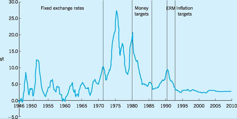
Fig. 22.1 Inflation is measured as the annual increase in the retail price index from 1946 to 1974, and in the retail price index excluding mortgage interest payments since 1974.
Source: ONS Economic Trends (various).
Comparing CPI and RPI indices
Although the CPI and RPI use roughly the same set of prices to construct each index, the results usually differ. The reasons for this difference are that they differ in coverage; the CPI covers a broader population base than the RPI; they differ in item coverage (specifically the CPI does not cover some housing costs); they have differing construction methodologies to combine prices into an overall index (the CPI uses a geometric mean, whereas the RPI uses an arithmetic mean). The difference between the two (CPI - RPI) was -1.5% points in September 2010, with some - 0.73 of the difference being explained by housing components excluded from the CPI, some -0.9 by the different construction methodologies, some +0.13 by the differences in the item coverage and some - 0.06 by other differences including weights.
As can be seen from Fig. 22.2 the percentage increase in inflation given by the RPI has usually been higher than that given by the CPI. Changing from the RPI to the CPI as the basis for upgrading benefits and public sector pensions is therefore controversial. Since 1990, £1,000 updated each year by the April RPI index would have amounted to £1,876 whereas £1,000 updated by the CPI would have amounted to only £1,615.
Other measures of inflation
No single inflation measure can meet all user needs. The Office for National Statistics (ONS) publishes several indices designed for specific purposes, some of which are explained below.
■ CPIY (Consumer Price Index excluding indirect taxes). CPIY is designed to measure ‘underlying’ price movements, but excluding those changes that are due to indirect tax changes such as VAT, and the duty on tobacco, alcohol and petrol.
In the year to September 2010 the CPIY rose by 1.5%.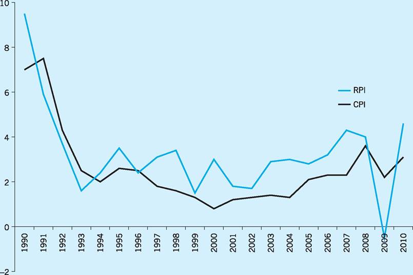
Fig. 22.2 CPI compared with RPI (all items) - annual percentage change. Source: ONS (various).
■ CPI-CT (Consumer Price Index at constant taxation). CPI-CT is an index where tax rates are kept constant at the rates that prevail in the base year. Comparing the CPI-CT to the CPI gives an indication of the impact of tax changes on the CPI. In the year to September 2010 the CPI-CT rose by 1.4%.
■ RPIX (Retail Price Index minus mortgage interest rates). RPIX was used to define the government inflation target prior to switching to the CPI in 2003. It is an attempt to get a picture of underlying inflationary pressure at a time when policy-makers might be using higher interest to subdue inflation. In the year to September 2010 RPIX rose by 4.6%.
■ RPIY (Retail Price Index minus direct taxes and mortgage interest rates). RPIY is an attempt to gauge core inflation excluding government initiated change in direct taxes and mortgage interest rates. In the year to September 2010 RPIY rose by 3.4%.
■ Tax and Price Index (TPI). TPI is a measure of how the average person’s gross income needs to change in order to buy a given basket of goods, allowing for income tax and national insurance changes. When these taxes rise, the TPI will rise faster than the RPI. It is useful to compare TPI with average earnings to indicate changes in the real purchasing power of gross earnings.
■ Pensioner indices. These are constructed to reflect the different purchasing pattern of pensioners. The single pensioner household index rose by 3.9% in the year 2009-2010.
■ Producer Price Index (PPI). PPI is a measure of the changes in price of goods bought and sold by UK manufacturers.
■ Services Products Providers Index (SPPI). SPPI is a measure of price changes in services provided by UK businesses to other UK businesses, and is thought to give some early indications of inflationary pressures.
European comparisons of inflation: the HICP
The Harmonized Index of Consumer Prices (HICP) is calculated in each EU country for purposes of comparison (it is the equivalent of the CPI in the UK). The European Central Bank aims to keep EU inflation below 2% as measured by the HICP though several EU countries have inflation rates well above this figure, including the UK (Table 22.2).
Low inflation as a policy objective
Much of the recent debate on inflation centres around how best to defeat it. Less is heard, at least in public debate, about the actual economic costs of inflation. It is important to identify these costs and to try and quantify them, so that they can then be compared with the costs of the policies aimed at reducing inflation. These latter costs are usually seen in terms of higher unemployment if restrictive monetary and fiscal policies are used to control inflation, or a misallocation of resources if prices and incomes policies are used. Traditionally the costs of inflation were seen in terms of its adverse effect on income distribution, as rising prices are particularly severe on those with fixed incomes, such as pensioners. However, Milton Friedman, in his Nobel lecture, shifted the focus of attention towards the adverse effects of inflation on output and employment.
In assessing the costs of inflation it is usual to distinguish two cases: that of perfectly anticipated inflation, where the rate of inflation is expected and has been taken into account in economic transactions, and that of imperfectly anticipated, or unexpected, inflation. We will consider perfectly anticipated inflation first, as it provides a useful benchmark against which to assess the more usual case of imperfectly anticipated inflation.
Table 22.2 HICP: EU comparisons of inflation (year to August 2010).
id="Picutre 189" class="lazyload" data-src="/files/uch_group77/uch_pgroup315/uch_uch7347/image/image178.jpg">
Source: ONS (2010) Consumer Price Indices Technical Manual.
Perfectly anticipated inflation
Suppose we initially have an economy in which inflation is proceeding at a steady and perfectly foreseen rate, and in which all possible adjustments for the existence of inflation have been made. In this economy all contracts, interest rates and the tax system would take the correctly foreseen rate of inflation into account. The exchange rate would also adjust to prevent inflation having any adverse effect on the balance of payments.
‘Shoe-leather' costs
In such an economy the main cost of inflation would arise from the fact that interest is not normally paid on currency in circulation. The opportunity cost to the individual of holding currency would then be the interest the individual could have earned on other assets, such as deposits at the bank. Higher anticipated inflation will tend to raise interest rates and therefore the opportunity cost of holding currency, with the rational response to this being for the individual to economize on currency holdings by making more frequent trips to the bank. The costs of these extra trips to the bank are often called the ‘shoe-leather’ costs of inflation. Although these costs are small for low rates of inflation, they have been estimated as rising to about 0.3% of GDP for perfectly anticipated inflation rates rising to around 10% per annum.
‘Menu' costs
A second cost, when inflation is fully anticipated, is that of having to change prices frequently. This is sometimes called the ‘menu’ cost of inflation. Presumably the more rapid the inflation, the more frequently things like price tags, cash tills, vending machines and price lists have to be changed, and this takes time, effort and money.
A study (Bakhshi et al. 1997) has attempted to estimate the benefits and costs of reducing perfectly anticipated inflation in the UK by 2% (which, given the current inflation target in the UK, would amount to achieving price stability). The annual welfare benefits of such a reduction in inflation were estimated at around 0.21% of GDP. Of course, the welfare benefits of lower inflation must be set against the lost output associated with the necessary deflation. Based on estimates of the UK ‘sacrifice ratio’ (the cost of cumulative lost output required for each percentage point reduction in inflation), Bakhshi et al. calculated the annual welfare loss of such a reduction in inflation to be around 0.18% of GDP. In other words, based on his estimates, there would be a net welfare gain of 0.03% of GDP per annum as a result of policies which reduce perfectly anticipated inflation in the UK by 2%.
Further costs arise from inflation when it is either not foreseen correctly, or not adjusted to fully. It is to these additional costs from imperfectly anticipated inflation that we now turn.
Imperfectly anticipated inflation
Redistribution effects
Unanticipated inflation leads to a redistribution of income and wealth. Debtors will gain at the expense of creditors if contracts do not take inflation fully into account and those on fixed incomes will suffer. In general there is likely to be a transfer from the private to the public sector. For example, inflation causes fiscal drag, taking individuals into higher tax brackets, thereby raising tax revenue for the public sector. Inflation also reduces the real value of the national debt, with government securities maturing at specified future dates for sums that are fixed in money terms, so that inflation reduces the real cost to the government of redeeming them. Inflation can, in effect, be regarded as an implicit tax on the holding of cash.
Costs of decision-taking
Uncertainty about future price levels is likely to lead to a misallocation of resources. For example, such uncertainty may discourage long-term contracts. This in turn is likely to inhibit investment which by its very nature tends to be long term. Savers and lenders may react to the uncertainty about future price levels by demanding a premium to cover the perceived extra risk. This premium will push up real interest rates and again discourage investment. Capital will also be misallocated if savers and investors form different expectations of inflation and hence different views as to expected real interest rates. There is evidence to suggest that the rate of inflation and the level of uncertainty are positively correlated (see Briault 1995).
Inflation and relative price movements
In market economies, changes in relative prices act as signals which serve to guide the allocation of resources. It is argued that economic agents find it difficult to discern relative price movements from general price level movements in times of inflation, especially when the rate of inflation is uncertain. In this case incorrect decisions will be made and resources will be misallocated.
The effects of inflation on economic growth
The previous analysis suggests that inflation (and especially uncertainty surrounding the future inflation rate) will lead to a misallocation of resources and a lower rate of economic growth. Testing this hypothesis empirically is extremely complex.
One approach is to use time-series data for single countries. Grimes (1991) found a significant negative relationship for 13 countries, which implied that a sustained increase in inflation from 0% to 9% would lead to a full percentage point reduction in annual growth rates. Others have found weaker but still negative relationships. The problem with simple regression equations used in such analyses is that it is difficult to get unbiased results. Difficulties arise in interpreting the overall negative relationship between inflation and growth. For example, in most countries, at least in the short run, inflation and economic growth are likely to be positively related, as in periods of boom. It might also be the case that the negative relationship might just be picking up the effects of policy measures; for example, a period of high inflation might precipitate a deflationary policy response which would slow the growth rate. The interested reader should consult Briault (1995) for further discussion of these issues.
An alternative approach is to use cross-country data. One example of this is the work done by Robert Barro (1995). He looked at data for 100 countries from 1960 to 1990. His regression results indicated that an increase in average inflation of 10% points per year reduces the growth or real per capita GDP by 0.2-0.3% points per year, and lowers the ratio of investment to GDP by 0.4-0.6% points. Although these effects may not appear particularly large, a reduction in growth rate of the above order of magnitude (brought about by a 10% rise in the average inflation rate) would mean that after 30 years real GDP would be 4-7% lower than otherwise. This would represent an estimated £30-50bn shortfall in GDP at current UK values of output.
Another study by Sarel (1996) suggested that the effect of inflation on growth is non-linear. He found a structural break in the relationship at an inflation rate of around 8%, with inflation below 8% per annum having no significant negative effects on growth, but inflation above 8% per annum having significant negative effects on growth, the suggestion here being that policy-makers should always keep inflation below the level (8%) consistent with this structural break.
A more recent study by Gillman and Harris (2010) of transition economies finds that inflation has a significant and negative effect on economic growth but that this effect decreases as the inflation rate rises. They conclude that monetary policy, via its effect on inflation, can therefore influence economic growth and suggest that the adoption of the low inflation Eurozone monetary policy or a monetary policy which sets a low target for inflation will be beneficial for these transition economies.
I Economic theory and inflation
The causes of inflation can be illustrated using the standard aggregate supply/demand framework found in most economic texts, such as Lipsey and Chrystal (1995) and Parkin et al. (2003). Figure 22.3 illustrates this framework. The first point to make is that the distinction between the short-run and long-run aggregate supply curves is important.
The upward sloping short-run aggregate supply (SRAS) curve assumes that some input prices, particularly money wages, remain relatively fixed as the price level changes. It then follows that an increase in the price level, whilst input prices remain relatively fixed, increases the profitability of production and induces firms to expand output and employ more labour. An increase in the general price level will therefore lead, in the short run, to some increase in real GDP.
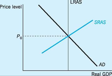
Fig. 22.3 Aggregate demand and supply.
There are two explanations as to why wages may remain constant even though prices have changed. First, many employees are hired under fixed-wage contracts. Once these contracts are agreed it is the firm that determines (within reason) the number of labour hours actually worked. If prices rise, the negotiated real wage will fall and firms will want to hire more labour time. Second, workers may not immediately be aware of price level changes, i.e. they may suffer from ‘money illusion’. If workers’ expectations lag behind actual price level changes, then workers will not be aware that their real wages have changed and will not adjust their wage demands appropriately. Both these reasons imply that as the price level rises, real wages will fall and the employment of extra labour hours will become more attractive to employers.
The long run is defined as the period in which all input prices (e.g. money wages) are fully responsive to changes in the price level. Workers in the long run can gather full information on price level changes and can renegotiate wage contracts in line with higher or lower prices. It follows that in the long run, a change in the price level is likely to be associated with an equal increase in money wages, leaving the real wage unchanged and by implication leaving employment and output unchanged. The long-run aggregate supply (LRAS) curve is independent of the price level; in other words, it is vertical.
Because, in the long run, all wages and prices can be renegotiated in line with supply and demand, the labour market will be in equilibrium (the real wage equating labour demand and supply) at the full employment level, with unemployment at the natural rate (see Chapter 23). The level of output associated with this level of employment is variously called the full employment level of output or the natural level of output. This level of output is obviously not constant but is determined by supply-side factors, such as the labour force, the capital stock and the state of technology. Through time this full employment or natural level of output can be expected to increase as the economy grows, i.e. the vertical LRAS curve can be expected to shift to the right.
Demand-pull inflation
One-off demand inflation
Consider the case of a one-off increase in aggregate demand. The source of the increase could be an increase in the money stock, an increase in the budget deficit, or any autonomous change in consumption, investment or net exports. Whatever the cause, the aggregate demand curve AD0 in Fig. 22.4 shifts to the right to AD1 along the short-run aggregate supply curve SRAS0. Excess demand now exists at the old price level P0 and this pushes prices up to P1. Such higher prices, with money wages lagging behind, increase the profitability of firms who then increase output beyond the full employment level Q0, so that unemployment falls below the natural rate. However, the new short-run equilibrium (B) with the output Q1 is not sustainable; labour is relatively scarce and workers will negotiate money wage increases to compensate for the increase in prices. The short-run aggregate supply curve now shifts up and to the left
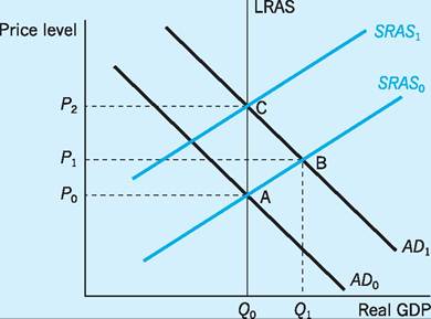
Fig. 22.4 A one-off increase in demand.
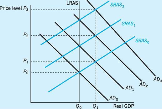
Fig. 22.5 Continuous demand inflation.
(i.e. from SRAS0 to SRAS1) in response to the increased costs of production, returning the economy to a new long-run equilibrium (C).
The economy experiences a period of ‘stagflation’ as output falls back to its natural level Q0 and the price level continues to rise to P2. The rise in price from P1 to P2 causing output to fall is usually explained in terms of rising prices reducing the real money supply, which in turn causes interest rates to rise and therefore interest-sensitive elements within aggregate demand to fall. Note that the inflation stops when the price level reaches P2. A one-off increase in aggregate demand will not therefore generate a lasting inflation.
Continuous demand inflation
Inflation proper, by which we mean a sustained upward movement in the price level, can occur only if the growth in aggregate demand is maintained. In this case output does not fall back to its natural rate but remains above it. It seems unlikely that autonomous shifts in private aggregate demand will be repeated period after period, which leaves either fiscal or monetary policy as the most likely cause of persistent demand inflation. However, expansionary fiscal policy, if funded by borrowing, is likely to lead to higher interest rates and therefore to the crowding-out of private spendings. This leaves monetary expansion as the most likely factor in turning a one-off inflation into a sustained inflation. The initial inflationary impulse could come from any demand-side factor, but an increase in the money supply is still necessary to prevent the price increases from reducing the real money supply, pushing up interest rates and eventually stopping the inflationary process. Figure 22.5 illustrates this case. As long as the money supply is allowed to expand in line with increasing prices, the aggregate demand curve continues to shift upward and the economy is kept above its natural level of output Q0. The cost of this money supply strategy, however, is continuing inflation, with the price level rising in each time period.
Cost-push inflation and supply shocks
Cost-push or supply-side inflation results from an increase in costs of production which firms pass on in the form of higher prices. The source of the cost increases could be a rise in imported raw material costs, such as the two oil price shocks of 1973-75 and 1979-80. Alternatively, trade unions may use their market power to push wages up irrespective of the pressure of demand in the labour market. In both these cases one group, OPEC or unions, is using market power to try and secure a larger share of output; firms, in response, attempt to protect their profits by increasing prices. Figure 22.6 shows cost-push/ supply-side inflation.
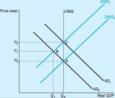
Fig. 22.6 Cost-push/supply-side inflation.
Suppose the economy is initially in equilibrium (A) with output at the full employment or natural rate Q0 and the price level at P0 with zero inflation. An increase in oil prices then shifts SRAS0, the short-run aggregate supply curve, to SRAS1. The economy now faces a period of stagflation with falling output, increased unemployment and rising prices. The period of stagflation ends when the new short-run equilibrium B is reached. If aggregate demand remains unchanged at AD0 then the excess supply in both goods and labour markets will eventually put downward pressure on costs and wages, causing the SRAS curve to return to its original position. This period of deflation returns the economy to its full employment equilibrium (A). However, this process is likely to be slow and painful, requiring a major adjustment in relative prices and a fall in real wages.
Expansionary monetary policy which shifts the aggregate demand curve to AD1 would speed up the process of returning the economy to full employment, but at the cost of additional inflation (Q0/P2 at point C). Indeed if the government got the timing and strength of the demand expansion just right, the economy could move from one long-run equilibrium to another, with very little loss of output. It is highly unlikely, however, that the government has the appropriate information and macroeconomic tools to stabilize output precisely at the full employment level Qo.
Continued cost-push inflation is unlikely, unless accompanied by accommodating monetary policy. Union pressure for wage increases would be undermined by falling output and increased unemployment, and even oil producers would eventually find that the reduced activity of non-oil-producers would restrict their market power. Monetary accommodation would, however, alter the story and might lead to repeated supply shocks and continuing inflation. Unions, thwarted in their attempt to seek real wage increases because of the higher prices associated with the monetary expansion and without the deterrent of unemployment, might ask for wage increases in the next round, causing the SRAS curve to shift to the left a second time. The choices for the government are, as before, either to allow unemployment to increase or to accommodate the new price increases by increasing the money supply and stimulating demand. The latter path could then lead to a continuous wage-price spiral.
There is no consensus as to the advisability of monetary accommodation of a supply-side shock. The policy decision depends to some extent on judging the relative costs to the state of extra unemployment against those of extra inflation. The danger with accommodation is that once inflationary expectations become entrenched in the wage-price setting process, they might be eliminated only after a prolonged period of unemployment (see the section on the Phillips curve below).
In conclusion, the theoretical analysis of inflation indicates that the government can always stop inflation, whether the cause is demand or supply-side factors. All the government has to do is to halt the growth of the money supply. The bad news, however, is that the cost of halting inflation is likely to entail a reduction in output and a rise in unemployment.
The relationship between inflation and unemployment (the Phillips curve)
Very few articles in economics have generated as much subsequent interest as A. W. Phillips' study of UK wage inflation and unemployment over the period 1861-1957. In the article (Phillips 1958) he appeared to find a stable and inverse relationship between unemployment and inflation (strictly, changes in wage rates). If unemployment was low, inflation would be high, and vice versa. The so-called Phillips curve suggested that with unemployment of around 5.5% there would be zero wage inflation and that with unemployment of around 2.5% the wage inflation generated would be covered by productivity growth, resulting in zero price inflation. This is depicted in Fig. 22.7. The relationship seemed to hold good over a long period of time and subsequent research found that it held good for many economies, and not just that of the UK.
The inverse relationship between inflation and unemployment was explained in terms of unemployment being an indirect measure of the level of excess demand in the economy. When unemployment is high and demand is low, the excess supply of labour holds wages and prices down; however, when unemployment is low and demand is high, the excess demand for labour will push wages and prices up more quickly. The Phillips curve appeared to offer the policy-maker a menu of choices from which could be chosen the preferred combination of unemployment and inflation, whilst at the same time highlighting the trade-off between the two policy objectives. If the economy was, say, at point A and the government wished to reduce unemployment by expanding aggregate demand, then it could do so but only at the cost of higher inflation, as at point B. Using the previous AD/AS framework, the expansionary fiscal or monetary policy would cause the AD curve to shift to the right, so that it now intersected further along the SRAS curve, thereby causing the price level to rise. The rise in prices will then push real wages down (because of either fixed contracts or workers' expectations lagging behind actual price increases), resulting in firms taking on more workers, unemployment falling and output rising. It is clear that some economists and policy-makers thought that point B could be maintained indefinitely if desired, but as we have seen and will confirm later, the existence of any such long-run trade-off (whereby a constant though
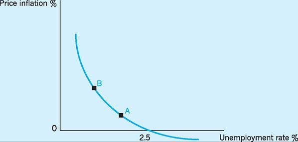
Fig. 22.7 The Phillips curve.
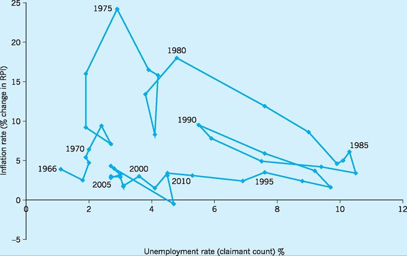
Fig. 22.8 The relationship between unemployment and inflation rates in the UK, 1966-2010. Source: ONS (various).
higher rate of inflation can be achieved for a given fall in unemployment) is highly questionable.
Breakdown of the Phillips curve
Evidence of the breakdown of the Phillips curve came very soon after the ‘discovery’ of this relationship that had supposedly been stable for over 100 years. Figure 22.8 plots UK inflation against unemployment since 1966. Clearly the downward sloping Phillips curve is not always in evidence in the period 19662010.
Supply-side factors
One reason why the Phillips relationship might not be entirely stable is the existence of supply-side inflation. As we have seen, raw material prices or wage increases may push costs and prices up irrespective of the pressure of demand, at least in the short term. In this case, a given level of unemployment would be associated with higher levels of inflation than the original Phillips curve would predict. The two oil price shocks of 1973-75 and 1979-80 resulted in periods of increased inflation that were not associated with falling unemployment, as the demand-side theory would have led us to predict.
Time-period factors
A more fundamental reason for the breakdown of the Phillips curve was proposed by Friedman (1968) and Phelps (1967). The new version of the Phillips curve makes the distinction between the short run and long run. It also assumes that markets are competitive enough in the long run to ensure that the real wage will be at the market clearing level. If this is the case, then labour supply will equal labour demand at the full employment level and unemployment will be at its natural rate. Note, however, that even when the market clears, not all workers who consider themselves to be part of the labour force will be either willing or able to accept a job at the going real wage. Some workers will be searching around for a better job offer (these are the frictionally unemployed), while other workers will not have the right skills or be in the right place (these are the structurally unemployed).
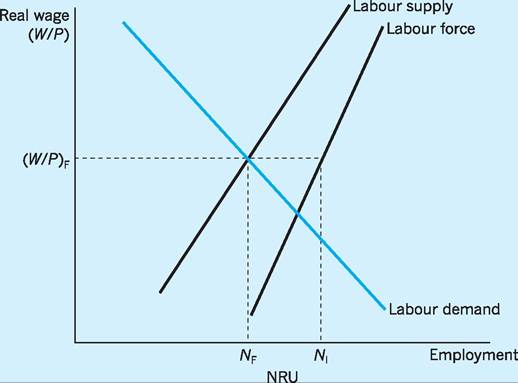
Fig. 22.9 The labour market.
The two groups together make up the natural rate of unemployment (NRU).
Figure 22.9 shows the market clearing or full employment real wage (W∕P)f and the associated full employment level of employment (Nf); the NRU is N1 - Nf, the difference between the amount of labour demanded and the labour force.
Expectational factors
The final strand of the revised Phillips curve is to emphasize the role of expectations in the inflationary process. Friedman pointed out that what workers and firms are interested in is the real wages, not the money wage. Wage bargaining takes place in money terms but when considering a money wage offer the expected inflation rate will be taken into account. The implication is that for any given level of unemployment (labour market tightness) there will be any number of possible money wage claims (for a given target real wage), depending on the expected level of inflation. As these money wage deals are passed on in price increases, it means that a given level of unemployment can be associated with any level of inflation which in turn means the existence of not just one Phillips curve but a whole family of Phillips curves, one for each expected inflation rate.
In Friedman’s view, once expectations are taken into account the unemployment/inflation trade-off is only a short-term possibility. Assume that the economy is currently at the natural rate of unemployment Un and that zero inflation has been experienced for some time and hence is expected to continue (point A in Fig. 22.10). The government attempts to increase output beyond the natural (full employment) rate by increasing the money supply. Aggregate demand shifts to the right and prices are forced up (as in Fig. 22.4 earlier). The increase in prices reduces real wages and so makes it profitable for firms to employ more labour. But why should previously unemployed labour take jobs they had previously rejected? As workers were expecting zero inflation, any money wage increase resulting from increased demand for labour will be interpreted as a real wage increase. As long as the money wage increase is less than the price increase, firms will be happy to employ the extra workers who have been ‘fooled’ into believing they have secured higher real wages by unexpectedly high inflation. Unemployment falls below the natural rate Un to Ub, and inflation increases to b as the economy moves along the shortrun Phillips curve (Ph0) to B. (Note: this is equivalent to a movement up and to the right along the shortrun aggregate supply curve in Fig. 22.4 earlier.)
If the inflation rate was to stay at b, workers would, sooner or later, adjust their inflationary expectations accordingly. Workers will then take the new and higher expected rate of inflation into account in their
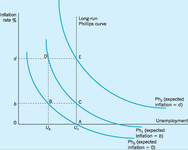
Fig. 22.10 The expectations-augmented Phillips curve.
wage bargains. This is equivalent to the short-run aggregate supply curve shifting up and to the left, and the Phillips curve shifting up and to the right (Ph1). The economy will now be at C, with unemployment and output falling back to their natural rates and with actual and expected inflation equal to b. In other words, C is a long-run equilibrium possibility, with an inflation rate constant at b.
Suppose, however, that the government wishes to return unemployment to Ub. It must then increase the growth of the money supply more rapidly, so that actual inflation again exceeds expected inflation. If the government does do this the economy will move along the new short-run Phillips curve to point D. As before, this short-run equilibrium cannot be maintained because expectations will again catch up with actual inflation, and the economy will then move to E as the short-run Phillips curve again shifts upwards (Ph2). At E the economy is once more in long-run equilibrium, with expected and actual inflation equal and the inflation rate constant at d.
Several interesting conclusions can be drawn from this modern view of the Phillips curve.
■ There is a short-run trade-off between unemployment and inflation but no long-run one.
■ Any rate of inflation is consistent with long-run equilibrium; all that is required is that expected inflation should equal actual inflation.
■ Attempts to push unemployment below the natural rate will result in increasing inflation. In fact the natural rate of unemployment is sometimes known as the non-accelerating inflation rate of unemployment (NAIRU).
■ Once inflationary expectations have become embedded in the system, a period of unemployment above the natural rate is required in order to lower the inflation rate. A movement down a given short-run Phillips curve to a level of unemployment above the natural rate will result in actual inflation being below expected inflation, leading to a downward revision of expectations, and hence falling inflation.
■ The natural rate of unemployment (and the NAIRU) are not constant over time. See Chapter 23 for a discussion of this issue.
UK inflationary experience: 1970-92
During the 1970s and early 1980s the UK experienced its highest periods of inflation in recent history. Inflation peaked in 1975, reaching nearly 27% (% change over the 12 months to August); then after falling back it peaked again in the year to June 1982, reaching 21.9%. Another period of inflation occurred in the year to September 1990 when inflation reached 10.9%.
The first of these three periods to 1975 was preceded by very buoyant aggregate demand, stimulated by money supply growth (as a result of relaxation of the rules on bank lending), an expansionary budget and a booming world economy. All these led to the AD curve shifting to the right beyond the full employment level of output and increasing inflation. This period of rapid demand-led growth can be seen in Fig. 22.11. Our analysis tells us that even without the adverse supply shock given by oil and other commodity prices in 1973, prices would have been given a further boost (and output would fall) as expectations of inflation were revised upwards in response to wage increases shifting the short-run AS curve up and to the left. The adverse supply shocks from oil and commodity price rises merely accelerated this process towards rising prices and falling output (note the fall in real GDP between 1973 and 1975 in Fig. 22.11).
The second inflationary episode occurred in the late 1970s and early 1980s. Again this period was marked by adverse supply shocks, including a doubling of oil prices, a near-doubling of VAT in 1979 (Q3) and an increase in wage costs, the last being the result of a catching-up process after a period of wage controls during 1974-79. The tightening of monetary and fiscal policy in late 1979 led to a further period of ‘stagflation’ in the following years (again note the fall in real GDP between 1979 and 1981 in Fig. 22.11).
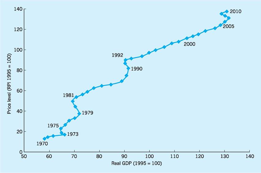
Fig. 22.11 UK price levels and real GDP, 1970-2010. Source: ONS and author's calculations.
It has been argued (Nelson and Nikolov 2002) that the reason why inflation was so troublesome in the late 1960s and the 1970s was partly due to policy-makers underestimating the degree of excess demand in the economy and partly due to the neglect of monetary policy. Underestimating the rate of productivity slowdown in the 1970s meant policymakers overestimated full employment output and hence underestimated the level of demand pressure (as measured by the output gap) in the economy. This was especially important over the 1972-74 period.
The reasons given for the neglect of monetary policy (meaning appropriate changes in interest rates) included:
■ the view held by some that inflation was caused by factors other than excess demand;
■ a feeling that incomes policy could be used as an alternative to demand management as a method of restraining inflation;
■ an assumption that cost-push inflation could continue indefinitely even in the absence of monetary accommodation (a view emanating from the Radcliffe Report of 1959 that argued that the velocity of circulation of money would adjust to offset any monetary policy); and
■ a scepticism about the impact of interest rates on aggregated demand.
Nelson and Nikolov conclude that if appropriate interest rate changes had been made and if the output gap had not been mismeasured, then the 9.3% points actual increase in average inflation from 1970 Q1 to 1979 Q1 compared to the 1960s could have been reduced by around 7.2% points.
The third inflationary episode was, like the first, associated with excess demand in the economy. Financial liberalization, a relaxation of monetary policy, rising house and other asset prices, growing consumer confidence, tax-cutting budgets in 1987 and 1988 and buoyant world demand all conspired to push aggregate demand beyond the full employment level. GDP was estimated to be over 4% above its full employment potential in both 1988 and 1989. Action to curtail inflation was taken in late 1988 when interest rates were increased by around 4% points to 12.8%. Further rate increases followed in 1989, but too little and too late to stop inflation rising to over 10% by the autumn of 1990.

Inflation targets and central bank independence 1992-
Since the early 1990s some 26 countries (including the UK, New Zealand, Canada, Australia and Brazil) have adopted explicit inflation targets. While the US has no explicit inflation target, the Federal Reserve Bank often indicates that it would prefer core inflation to be around 2%, similar to the inflation target in the Eurozone, with the European Central Bank aiming for inflation of below but close to 2%. Instead of using intermediate policy targets, such as the money supply or the exchange rate to achieve inflation stability, the emphasis has moved towards the use of explicit inflation targets. In the UK the initial inflation target set in 1992, by the then government, was 2.5% as measured by the RPIX; this was later replaced by the current target of 2% as measured by the CPI. A further significant change occurred in 1997 when the government delegated the power to decide interest rates to the nine member MPC of the Bank of England (see Chapter 20). The MPC is charged with setting short-term interest rates in order to meet the government’s inflation target in the medium term. Put simply, if the MPC forecasts that the CPI is going to be above 2% in approximately two years’ time (given the time lags before interest rates have their maximum impact), it might seek to raise interest rates now to bring future inflation back into line. The inflation target is a symmetrical one, in that inflation below 2% is regarded as being just as undesirable as inflation above 2%, so that interest rates will be lowered if an inflation rate below target is forecast.
The UK framework has been intended to remove politics from interest rate decision-making, as these decisions are taken by the independent MPC and should give monetary policy more credibility and help keep inflationary expectations around the official target. Credibility is also enhanced by increased transparency and accountability. The publication of the Quarterly Inflation Report and the Minutes of the monthly MPC meetings improves transparency and the requirement for the Governor of the Bank of England to write a letter of explanation if actual inflation rate deviates by more than 1% from the target (in either direction) helps ensure accountability. The first such letter had to be written in April 2007 after the March inflation rate had risen to
Table 22.3 UKinflation dynamics, 1950-2007.
| Period | Mean | Standard deviation | Persistence* |
| Jan 1950-April 1997 | 6.1 | 5.1 | 0.7 |
| May 1997-March 2007 | 1.5 | 0.5 | 0.5 |
*Persistence is the correlation co-efficient between inflation in December of the year in question and inflation the previous December.
Source: King (2007).
3.1%. In August 2010 the Governor again explained in a written letter that the inflation rate of 3.1% for the year to July 2010 was due to the VAT increase in January, to past increases in the oil price and to the continued impact of Sterling depreciation since 2007 on import prices. However, given that the impact of these should diminish by the time of the next 12-month comparison and given that there is considerable spare capacity in both product and labour markets, the then Governor felt able to forecast that, although inflation would be above target until the end of 2011, it would fall back to the target level after that and so no change needs to be made to the current interest rate.
The current Governor of the Bank of England, Mervyn King, reviewed the effectiveness of the UK inflation framework in 2002 and 2007. He found that inflation in the UK since the mid-1990s had been lower than for a generation; less variable and less persistent (see Table 22.3). He also pointed out that the lower and more stable inflation rate was not at the expense of a restricted demand and lower economic growth. The average growth rate of the UK economy (1997-2007) at 2.8% per annum was above the post-war average and better than that in any G7 country apart from Canada, as compared with the period 1950-1996 when the UK had the lowest recorded G7 growth rate.
A key question is whether the change in the monetary policy framework has been the cause of low inflation and stability in the real economy, or whether the causation runs from a more stable world environment (at least up to 2007) resulting in lower inflation! King (2007) argues that the better outcomes for inflation and economic stability are not simply the result of luck but that the crucial achievement of the new monetary policy framework has been to anchor inflationary expectations at a low level, with the result that monetary policy is not adding to the volatility of the economy as it sometimes did in previous decades.
Conclusion
It is generally agreed that the high and volatile UK inflation experience of the 1970s and 1980s did substantial harm to the UK economy. In the medium term, inflation is determined by the balance between aggregate expenditure and supply-side capacity. The new inflation framework has been relatively successful in controlling expenditure and hence in keeping inflation in check. Low and stable inflation (however defined) may be insufficient on its own to guarantee continued macroeconomic stability, but it is likely to remain as a central objective of monetary policy in the medium- and long-run time periods. Short-run variations of actual inflation from target inflation are inevitable, being caused by unpredictable factors such as sudden VAT increases, oil price increases and currency depreciations. These factors are not easily influenced by interest rates and their impacts on inflation should be largely ignored as long as the medium-term forecast for inflation is that it will return to its target level.
In the light of the recent financial crisis, however, adjustments to the current inflation framework have been considered. Nevertheless, there is widespread agreement at present that the alternatives undermine either the simplicity or the credibility of the current inflation framework that are so important in anchoring inflationary expectations with the current inflation framework still the best available.
Key points
■ The RPI measures movement in the prices of a ‘basket’ of goods and services bought by a representative UK household.
■ Items with higher income elasticities of demand (e.g. housing, leisure services, catering) are being given increasing weights in the calculation of the RPI.
■ The RPI is linked back to January 1987 = 100 as base. With an RPI of 225.3 in September 2010, this indicates that average retail prices have risen by 125.3% since January 1987.
■ RPIX is RPI excluding mortgage interest payments.
■ RPIY is RPI excluding mortgage interest payments and indirect taxes.
■ The CPI replaced the RPIX as the UK inflation target in 2003.
■ The modern view of the Phillips curve is that there is a short-run trade-off between unemployment and inflation, but no long-run trade-off.
■ Attempts to push unemployment below the natural rate will result in increasing inflation.
■ This natural rate of unemployment is sometimes known as the non-accelerating inflation rate of unemployment (NAIRU).
■ The government sets the inflation target and the Monetary Policy Committee (MPC) changes interest rates in trying to meet that target.
■ There is evidence that setting an inflation target may itself help to reduce inflation without inhibiting growth.
Now try the self-check questions for this chapter on the Companion Website. You will also find useful links to relevant websites.
Note
1 Using chain indexing - the index for, say, May 2007 with base year 2005 is given by:
Index May, 2007 | 2005 = Index Dec 2006 | 2005 ? Index Jan 2007 | Dec 2006 ? Index May, 2007 | Jan 2007
References and further reading
Bakhshi, H., Haldane, A. and Hatch, N. (1997) Some costs and benefits of price stability in the UK, Bank of England Quarterly Bulletin, 37(3): 274-84.
Barro, R. (1995) Inflation and economic growth, Bank of England Quarterly Bulletin, 35(2): 166-76.
Bean, C., Paustian, M., Penalver, A. and Taylor, T. (2010) Monetary policy after the fall, Federal Reserve Bank of Kansas City Conference, Jackson Hole, WY, 26-28 August.
Benassy-Quere, A. and Coeure, B. (2010) Economic Policy, Oxford, Oxford University Press. Briault, C. (1995) The costs of inflation, Bank of England Quarterly Bulletin, 35(1): 33-5. Cobham, D. (2010) Twenty Years of Inflation Targeting Lessons Learned and Future Prospects, Cambridge, Cambridge University Press.
Dungey M., Fry, R., Gonzales-Hermosillo, B. and Martin, V. (2011) Transmission of Financial Crises and Contagion, Oxford, Oxford University Press.
Friedman, M. (1968) The role of monetary policy, American Economic Review, 58(March): 1-17.
Friedman, M. (1977) Inflation and unemployment, Journal of Political Economy, 85(3): 451-72.
Giavazzi, F. and Blanchard, O. (2010) Macroeconomics: A European Perspective, Harlow, Financial Times/Prentice Hall.
Gillman, M. and Harris, M. (2010) The effect of inflation on growth. Evidence from a panel of transition countries, Economics of Transition, 18 (4): 678-714.
Gnos, C. (2009) Monetary Policy and Financial Stability, Cheltenham, Edward Elgar.
Grimes, A. (1991) The effects of inflation on growth: some international evidence, Weltwirtschaftliches Archive, 127: 631-44.
IMF (2006) How has globalization affected inflation? World Economic Outlook, April, Washington DC, International Monetary Fund. King, M. (2002) The inflation target ten years on, lecture delivered at the London School of Economics, 19 November 2002, Bank of England Quarterly Bulletin, 42 (4), Winter.
King, M. (2007) The MPC Ten Years On, lecture delivered to the Society of Business Economists, London, 2 May.
Lipsey, R. and Chrystal, K. (1995) Positive Economics, Oxford, Oxford University Press. Nelson, E. and Nikolov, K. (2002) Monetary Policy and Stagflation in the UK, Working Paper No. 155, May, London, Bank of England. Nickell, S. (2006) Monetary Policy, Demand and Inflation, speech given to Bank of England South East and East Anglia Agency, 31 January 2006.
ONS (2010) Consumer Price Indices Technical Manual, London, Office for National Statistics.
Parkin, M., Powell, M. and Matthews, K. (2003) Economics, London, Addison Wesley Longman. Phelps, E. S. (1967) Phillips curves, expectations of inflation and optimal unemployment over time, Economica, 34(August): 254-81.
Phillips, A. W. (1958) The relation between unemployment and the rate of change of money wage rates in the United Kingdom, Economica, 25(November): 283-99.
Radcliffe Committee (1959) Report on the Working of the Monetary System, CMND. 827, London, HMSO.
Sarel, M. (1996) Nonlinear effects of inflation on economic growth, IMF Staff Papers, 43(1): 199-215.
Soteri, S. and Westaway, P. (1993) Explaining price inflation in the UK: 1971-92, National Institute Economic Review, 144(May): 85-94.
More on the topic Inflation:
- The Phillips Curve and Inflationary Expectations
- CHAPTER SUMMARY
- REVIEW QUESTIONS
- REVIEW QUESTIONS
- NUMERICAL PROBLEMS
- Conclusion
- Conclusion
- Conclusion
- KEY EQUATION
- Macroeconomics focuses on the analysis of economies in their entirety.