The IS-LM Model for an Open Economy

Use the relationship between exchange rates and international trade to develop an open-economy IS-LM model.

Now we're ready to explore how exchange rates and international trade interact with the behavior of the economy as a whole.

Recall that the components of the IS-LM model are the IS curve, which describes goods market equilibrium; the LM curve, which describes asset market equilibrium; and the FE line, which describes labor market equilibrium. Nothing discussed in this chapter affects our analysis of the supply of or demand for money in the domestic asset market; so, in developing the open-economy IS-LM model, we use the same LM curve that we used for the closed-economy model. Similarly, the labor market and the production function aren't directly affected by interna­tional factors, so the FE line also is unchanged.^[243]

However, because net exports are part of the demand for goods, we have to modify the IS curve to describe the open economy. Three main points need to be made about the IS curve in the open economy:

1. Although the open-economy IS curve is derived somewhat differently than the closed-economy IS curve, it is a downward-sloping relationship between output and the real interest rate, as the closed-economy IS curve is.

2. All factors that shift the IS curve in the closed economy shift the IS curve in the open economy in the same way.

3. In an open economy, factors that change net exports also shift the IS curve. Specifically, for given values of domestic output and the domestic real interest rate, factors that raise a country's net exports shift the open-economy IS curve up and to the right; factors that lower a country's net exports shift the IS curve down and to the left.

After discussing each point, we use the open-economy IS-LM model to ana­lyze the international transmission of business cycles and the operation of macro­economic policies in an open economy.

The Open-Economy /S Curve

For any level of output the IS curve gives the real interest rate that brings the goods market into equilibrium. In a closed economy, the goods market equilib­rium condition is that desired national saving, S^d, must equal desired investment, I^d, or S^d — I^d = 0. In an open economy, as we showed in Chapter 5, the goods market equilibrium condition is that desired saving, S^d, must equal desired invest­ment, I^d, plus net exports, NX. Writing the goods market equilibrium condition for an open economy, we have

S^d — I^d = NX. (13.4)

FIGUREJ3.5

Goods market equilibrium in an open economy

The upward-sloping curve shows desired saving, S^d, less desired investment, I^d. This curve slopes upward because a higher domestic real interest rate increases the excess of desired saving over desired investment. The NX curve relates net exports to the domestic real interest rate. This curve slopes downward because a higher domes­tic real interest rate causes the real exchange rate to appreciate, reduc­ing net exports. Goods market equilibrium occurs at point E, where the excess of desired sav­ing over desired invest­ment equals net exports (equivalently, where desired lending abroad equals desired borrowing by foreigners). The real interest rate that clears the goods market is r₁.

To interpret Eq. (13.4), recall that S^d — I^d, the excess of national saving over invest­ment, is the amount that domestic residents desire to lend abroad. Recall also that net exports, NX (which, if net factor payments and net unilateral transfers are zero, is the same as the current account balance), equals the amount that foreigners want to borrow from domestic savers.

Equivalently, we can write the goods market equilibrium condition as

We obtained Eq. (13.5) from Eq. (13.4) by replacing desired saving, S^d, with its definition, Y — C^d — G, and rearranging. Equation (13.5) states that the goods market is in equilibrium when the supply of goods, Y, equals the demand for goods, C^d + I^d + G + NX. Note that in an open economy the total demand for goods includes spending on net exports.

Figure 13.5 illustrates goods market equilibrium in an open economy. The horizontal axis measures desired saving minus desired investment, S^d — I^d, and net exports, NX. Note that the horizontal axis includes both positive and negative values. The vertical axis measures the domestic real interest rate, r.

The upward-sloping curve, S^d — I^d, shows the difference between desired national saving and desired investment for each value of the real interest rate, r. This curve slopes upward because, with output held constant, an increase in the real interest rate raises desired national saving and reduces desired investment, raising the country's desired foreign lending.

The downward-sloping curve, NX, in Fig. 13.5, shows the relationship between the country's net exports and the domestic real interest rate, other factors held constant. As discussed in Section 13.2, a rise in the real interest rate appreciates the exchange rate, which in turn reduces net exports (see Summary table 17). Hence the NX curve slopes downward.

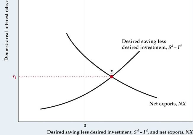
Goods market equilibrium requires that the excess of desired saving over desired investment equal net exports (Eq.

To derive the open-economy IS curve, we need to know what happens to the real interest rate that clears the goods market when the current level of domestic output rises (see Figure 13.6). Suppose that domestic output initially equals Y₁ and that goods market equilibrium is at point E, with a real interest rate of r₁. Now suppose that output rises to Y₂. An increase in current output raises desired national saving but doesn't affect desired investment, so the excess of desired sav­ing over desired investment rises at any real interest rate. Thus the curve measur­ing the excess of desired saving over desired investment shifts to the right, from (S^d — I^d )¹ to (S^d — I^d )² in Fig. 13.6(a).

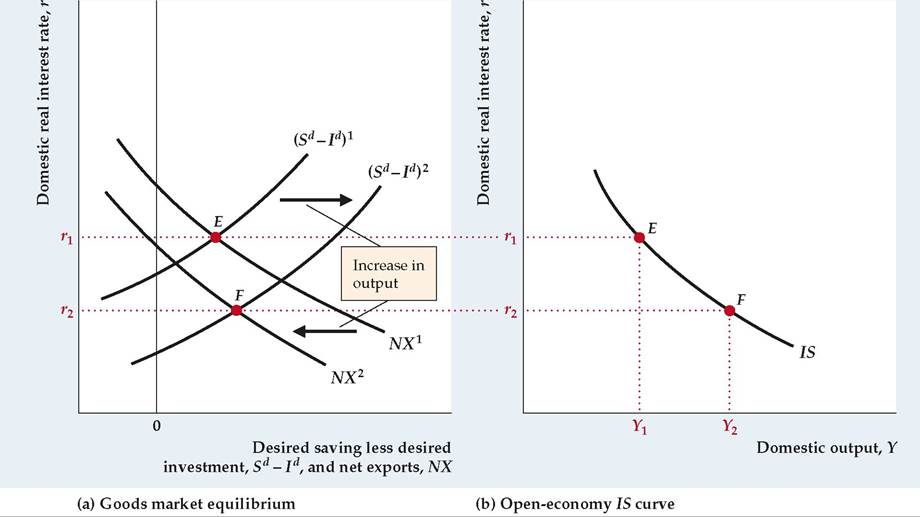
FIGURE 13.6

Derivation of the /S curve in an open economy

The initial equilibrium in the goods market is represented by point E in both (a) and (b).

(a) At point E, domestic output is Y₁ and the domestic real interest rate is r₁. An increase in domestic output from Y₁ to Y₂ raises desired national saving at each real interest rate and doesn't affect desired investment. Therefore the S^d — I^d curve shifts to the right, from (S^d — I^d )¹ to (S^d — I^d )². The increase in output also raises domestic spending on imports, reducing net exports and causing the NX curve to shift to the left, from NX¹ to NX². At the new equilibrium point, F, the real interest rate is r₂.

(b) Because an increase in output from Y₁ to Y₂ lowers the real interest rate that clears the goods market from r₁ to r₂, the IS curve slopes downward.

What about the NX curve? An increase in domestic income causes domestic consumers to spend more on imported goods, which (other factors held constant) reduces net exports (Summary table 17). Thus, when output rises from Y₁ to Y₂, net exports fall, and the NX curve shifts to the left, from NX¹ to NX².

After the increase in output from Y₁ to Y₂, the new goods market equilibrium is at point F in Fig. 13.6(a), with the real interest rate at r₂. The IS curve in Fig. 13.6(b) shows that, when output equals Y₁, the real interest rate that clears the goods market is r₁; and that when output equals Y₂, the real interest rate that clears the goods market is r₂. Because higher current output lowers the real interest rate that clears the goods market, the open-economy IS curve slopes downward, as for a closed economy.

Factors That Shift the Open-Economy /S Curve

As in a closed economy, in an open economy any factor that raises the real interest rate that clears the goods market at a constant level of output shifts the IS curve up. This point is illustrated in Figure 13.7 which shows the effects on the open-economy IS curve of a temporary increase in government purchases. With

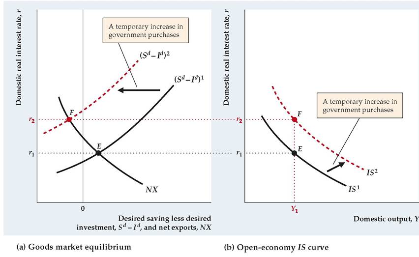
FIGURE 13.7

Effect of an increase in government purchases on the open-economy /S curve

Initial equilibrium is at point E, where output is Y₁ and the real interest rate is r₁, in both (a) and (b).

(a) A temporary increase in government purchases lowers desired national saving at every level of output and the real interest rate. Thus the S^d — I^d curve shifts to the left, from (S^d — I^d )¹ to (S^d — I^d )².

(b) For output Y₁, the real interest rate that clears the goods market increases to r₂, at point F in both (a) and (b).

output held constant at Y₁, the initial equilibrium is at point E, where the real interest rate is r₁. A temporary increase in government purchases lowers desired national saving at every level of output and the real interest rate. Thus the S^d — I^d curve shifts to the left, from (S^d — I^d )¹ to (S^d — I^d )², as shown in Fig. 13.7(a). The new goods market equilibrium is at point F, where the real interest rate is r₂.

Figure 13.7(b) shows the effect on the IS curve. For output Y₁, the increase in government purchases raises the real interest rate that clears the goods market from r₁ to r₂. Thus the IS curve shifts up and to the right, from IS¹ to IS².

In general, any factor that shifts the closed-economy IS curve up does so by reducing desired national saving relative to desired investment. Because a change that reduces desired national saving relative to desired investment shifts the S^d — I^d curve to the left (Fig. 13.7a), such a change also shifts the open-economy IS curve up.

In addition to the standard factors that shift the IS curve in a closed economy, some new factors affect the position of the IS curve in an open economy. In par­ticular, anything that raises a country's net exports, given domestic output and the domestic real interest rate, will shift the open-economy IS curve up. This point is illustrated in Figure 13.8.

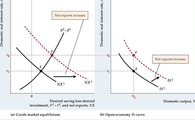
FIGURE 13.8

Effect of an increase in net exports on the open-economy /S curve

In both (a) and (b), at the initial equilibrium point, E, output is Y₁ and the real interest rate that clears the goods market is r₁.

(a) If some change raises the country's net exports at any given domestic output and domestic real interest rate, the NX curve shifts to the right, from NX¹ to NX 2.

(b) For output Y₁, the real interest rate that clears the goods market has risen from r₁ to r₂, at point F in both (a) and (b). Thus the IS curve shifts up and to the right, from IS¹ to IS².

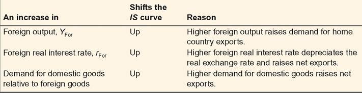
SUMMARY 18

International Factors That Shift the /S Curve

At the initial equilibrium point, E, in both Figs. 13.8(a) and (b), domestic out­put is Y₁ and the domestic real interest rate is r₁. Now suppose that some change raises the country's net exports at any level of domestic output and the domestic real interest rate. This increase in net exports is shown as a shift to the right of the NX curve in Fig. 13.8(a), from NX¹ to NX². At the new goods market equilibrium point, F, the real interest rate has risen to r₂. Because the real interest rate that clears the goods market has risen for constant output, the IS curve shifts up and to the right, as shown in Fig. 13.8(b), from IS¹ to IS².

What might cause a country's net exports to rise, for any given domestic out­put and domestic real interest rate? We've discussed three possibilities at various points in this chapter: an increase in foreign output, an increase in the foreign real interest rate, and a shift in world demand toward the domestic country's goods (see Summary table 17).

■ An increase in foreign output, Y_For, increases purchases of the domestic country's goods by foreigners, directly raising the domestic country's net exports and shifting the IS curve up.

■ An increase in the foreign real interest rate, r_For, makes foreign assets relatively more attractive to domestic and foreign savers, increasing the supply of domestic currency and reducing the demand for domestic currency, thereby causing the exchange rate to depreciate. A lower real exchange rate stimulates net exports, shifting the domestic country's IS curve up.

■ A shift in world demand toward the domestic country's goods, as might occur if the quality of domestic goods improved, raises net exports and thus also shifts the IS curve up. A similar effect would occur if, for example, the domestic country imposed trade barriers that reduced imports (thereby increasing net exports); see Analytical Problem 1 at the end of the chapter.

Summary table 18 lists factors that shift the open-economy IS curve.

The International Transmission of Business Cycles

In the introduction to this chapter we discussed briefly how trade and financial links among countries transmit cyclical fluctuations across borders. The analysis here shows that the impact of foreign economic conditions on the real exchange rate and net exports is one of the principal ways by which cycles are transmitted internationally.

For example, consider the impact of a recession in the United States on an econ­omy for which the United States is a major export market—say, Japan. In terms of the IS-LM model, a decline in U.S. output lowers the demand for Japanese net exports, which shifts the Japanese IS curve down. In the Keynesian version of the model, this downward shift of the IS curve throws the Japanese economy into a recession, with output below its full-employment level, until price adjustment restores full employment (see, for example, Fig. 11.7). Japanese output also is pre­dicted to fall in the classical model with misperceptions because the drop in net exports implies a decline in the Japanese aggregate demand (AD) curve and the short-run aggregate supply (SRAS) curve slopes upward. However, in the basic classical model without misperceptions, output remains at its full-employment level so the decline in net exports wouldn't affect Japanese output.

Similarly, a country's domestic economy can be sensitive to shifts in interna­tional tastes for various goods. For example, a shift in demand away from Japanese goods—induced perhaps by trade restrictions against Japanese products—would shift the Japanese IS curve down, with the same contractionary effects as the decrease in foreign (U.S.) output had.

13.4