The Samuelson Multiplier Accelerator Model

All versions of the Keynesian model we have considered so far are essentially static short-run equilibrium models. In an important paper, Samuelson [1939] combined the model of the Keynesian cross with an investment function based on the principle of acceleration to derive a dynamic model of endogenous business cycles.

Samuelson considered the following dynamic version of the model of the Keynesian cross:

where a, b, c, d, and e are constant parameters; a is the accelerator, which determines how a change in consumption affects current investment; b is autonomous investment; c < 1 is the marginal propensity to consume; and d is autonomous consumption. Finally, e is government expenditure, assumed exogenous and constant.

The investment function (15.14) is based on the so-called acceleration principle, which implies that when there is a positive change in consumption, firms will invest more to produce the higher quantity of consumer goods demanded. When there is a negative change in consumption, firms will reduce investment, as they need less capital to meet the lower demand for consumer goods. The accelerator a measures the sensitivity of investment to changes in aggregate consumption.¹⁶

Equation (15.15) is a linear Keynesian consumption function, according to which consumption is a function of lagged and not current income. Government expenditure is assumed exogenous and constant at e. Substituting (15.15) in (15.14), the investment function can be written as

Investment is a function of the lagged change in income, as the lagged change in income drives the demand for consumption goods.

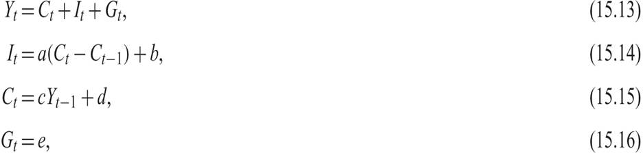
Substituting the consumption function (15.15), the investment function (15.17), and (15.16) in the equilibrium condition of the market for goods and services (15.13), after collecting terms, one gets

The dynamic path of output in the Samuelson [1939] model is thus determined by the second-order difference equation (15.18).

The particular solution of this equation, which defines equilibrium output, is given by

Equilibrium output depends only on autonomous expenditure and the multiplier 1/(1 −c), as suggested by the model of the Keynesian cross. However, the dynamic path of output is determined by the difference equation (15.18), which also depends on the accelerator.¹⁷

For the difference equation (15.18) to be stable, ac must be less than one, or the accelerator must satisfy a < 1/c. If this condition is not satisfied, output will not converge to equilibrium but instead will diverge.

For the roots to be real, we must have c ≥ 4a/(1 + a)². Thus, for the roots to be real and for income to converge monotonically to its equilibrium value, the condition is

For (15.20) to be satisfied, if the marginal propensity to consume is equal to three-quarters (0.75), the accelerator must be less than or equal to one-third (0.333). In such a case, the difference equation will converge monotonically.

If the accelerator is such that the inequality on left-hand side of (15.20) is strict, the roots will be real, distinct, and less than one. The general solution of (15.18) will then take the form

where Y₁, Y₂ are two boundary (initial conditions).

Real output will converge monotonically to its equilibrium level Y^*, which is given in (15.19).

If the left-hand side of (15.20) is equal to c, then we have two repeated roots, λ = c(1 + a)/2 < 1. The general solution of (15.18) then takes the form

Real output will converge monotonically to its equilibrium level Y^*, which is given (15.19).

In the case where the inequality on the left-hand side of (15.20) is not satisfied, then we have two complex roots λ₁, λ₂, and real output will display damped oscillations (i.e., endogenous fluctuations) during the convergence to its equilibrium value. This will occur as long as a < 1/c. If the accelerator does not satisfy this condition, then the model displays divergent oscillations.

The complex roots will take the form of a pair of complex conjugates of the form

where , and 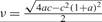. The general solution will then take the form

where θ is defined by

This solution will display oscillations of a periodic nature. Because we have assumed that ac < 1, the oscillations will be dampened, and there will be cyclical convergence to the equilibrium value given by (15.19).

Figure 15.6 shows the dynamic convergence of real output for different values of the accelerator, assuming that the equilibrium value is equal to zero. We assume that c = 0.75, and that the accelerator takes three alternative values: (1) a = 1/10, (2) a = 1/3, and (3) a = 11/10. Case 1 results in two real and distinct rules, and monotonic convergence to equilibrium. Case 2 results in repeated real roots and monotonic convergence to equilibrium. Case 3 results in complex roots and cyclical convergence to equilibrium. Thus, if the accelerator is sufficiently high in this model, cyclical convergence (i.e., cyclical fluctuations) occurs.

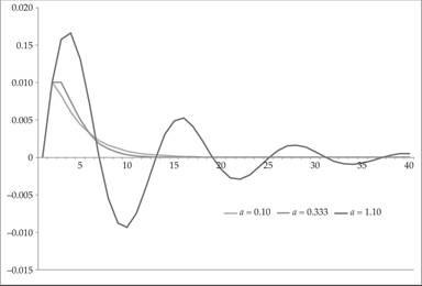
Figure 15.6 Convergence of real output for different values of the accelerator.

15.3