The Original Keynesian Models

In the analysis of the General Theory, and subsequent Keynesian models, the assumption of the immediate adjustment of wages and prices to equilibrate labor and product markets was replaced by the assumption that there is a short-term rigidity in their adjustment, and that the short-run macroeconomic adjustment mechanism also involves quantities such as the level of real income and employment.³

In this section, we look at the three main forms of the original Keynesian model.

15.1.1 The Keynesian Cross

The Keynesian model starts by considering the determination of aggregate demand. The assumption is that total real output and income Y is determined by aggregate demand, consisting of real consumption C, real gross investment I, and real government expenditure G:

In the simplest version, that of the Keynesian cross, investment and government expenditure are considered exogenous, and the only behavioral equation is the consumption function. Consumption is assumed to be a positive function of current real disposable income:

where T denotes the real value of taxes, and the first derivative of the consumption function satisfies

The parameter C_Y is termed the marginal propensity to consume and is assumed to be less than unity.

Keynes [1936] devoted a significant number of pages in chapters 8 and 9 of the General Theory to the justification of the consumption function. Also, note that the Keynesian consumption function differs radically from the Euler equation for consumption we have been relying on so far. It focuses on disposable household income as the main determinant of consumption and explicitly denies a role for the interest rate.⁴

From (15.1) and (15.2), we can determine the equilibrium condition between total output and aggregate demand, which is the equilibrium condition in the market for goods and services:

The equilibrium condition (15.3) is depicted in figure 15.1, which is also known as the Keynesian cross.⁵

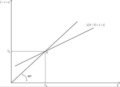
Figure 15.1 Exogenous investment and government expenditure: the Keynesian cross.

Real output is determined by the equality of aggregate supply and aggregate demand, which is the sum of real consumption, investment, and government expenditure. Prices are assumed to be fixed or sluggish to adjust. Therefore, a change in aggregate demand induces firms to produce more and thus brings about a change in aggregate output and employment.⁶

From equation (15.3), one can derive the multiplier:

An exogenous change in aggregate demand, either through investment or through government expenditure, results in a change in real output that is a multiple of the original change. The multiple is determined by the multiplier, which is the inverse of the marginal propensity to save: 1 − C_Y.

When aggregate demand increases because of an autonomous increase in investment or real government expenditure, real output and income initially increases by the same amount. This increase in real output and income induces an increase in private consumption through the consumption function, which brings about a further increase in aggregate demand, real output, and employment. Consequently, a given exogenous rise in aggregate demand has a compound effect on aggregate real income, due to the second (and subsequent) round effects through aggregate consumption. These produce further increases in real demand, real output, and employment, further rises in private consumption, and so on.⁷

From equation (15.3), one can also derive the balanced budget multiplier, that is, the effect of a change in government expenditure and taxes that leaves the budget deficit unchanged. Under the assumption that dG_t = dT_t, it follows that

An increase in public expenditure, funded by an equal increase in taxes, increases total aggregate expenditure, real output, and income by the same amount. This is something that was proven by Haavelmo [1945]. Government expenditure increases aggregate demand one-to-one, but the tax increase reduces private consumption by less than one-to-one, because the marginal propensity to consume is less than one. Consequently, the initial impact on aggregate expenditure is 1 − C_Y, the inverse of the multiplier, and the overall effect of a change in government expenditure financed by increased taxes is equal to unity.

The model of the Keynesian cross assumes that investment is exogenous. In an important paper, Samuelson [1939] combined this model with an investment function based on the principle of acceleration to derive endogenous business cycles in the Keynesian model.

15.1.2 The IS-LM Model

A more general form of the basic Keynesian model considers that aggregate investment depends on the real interest rate and introduces the equilibrium condition in the market for money to analyze the simultaneous determination of real output and the interest rate. This form is analyzed in chapters 10–18 of Keynes [1936], and was codified as the IS-LM model, in an important paper by Hicks [1937].⁸

The main difference from the previous model of the Keynesian cross is that investment ceases to be treated as exogenous, and is considered to depend negatively on the real interest rate. Assuming that inflationary expectations are given, investment will depend negatively on the current nominal interest rate. Consequently, the equilibrium condition in the goods and services market takes the form⁹

where i is the nominal interest rate. The effect of the nominal interest rate on investment is assumed to be negative:

Equation (15.6) describes the combinations of real output and the nominal interest rate that ensure equilibrium in the market for goods and services. It is depicted as the downward-sloping investment-savings (IS) curve in figure 15.2.

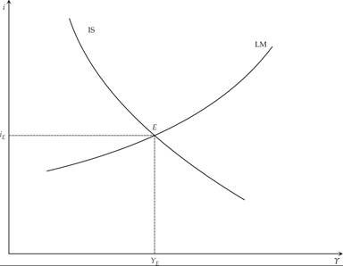
Figure 15.2 Aggregate output and the nominal interest rate: the IS-LM model.

When a new endogenous variable (the nominal interest rate) is introduced, one should analyze how it is determined. This is done through introducing the equilibrium condition in the money market.

where M is the nominal money supply, P the price level (which is considered as given in this version of the model), and m the demand function for real money balances (liquidity preference, in the terminology of Keynes).

The properties of the money demand function are described by

Equation (15.7) describes the combinations of real output and the nominal interest rate that are consistent with equilibrium in the money market, in the sense that money demand is equal to the exogenous money supply for the given price level. It is depicted as the upward-sloping LM (liquidity-money) curve in figure 15.2.

Real output and the nominal interest rate are determined at the point where both the market for goods and services and the market for money are in equilibrium. At the point of intersection of the IS curve (which describes equilibrium in the market for goods and services) and the LM curve (which describes equilibrium in the money market), the economy is thus in short-run equilibrium. Because the price level is assumed to be fixed, this equilibrium can occur at less than full employment. In fact, this is the assumption usually made in Keynesian models.

It is simple to deduce that an increase in government expenditure or a tax cut shifts the IS curve to the right and causes an increase in real output and the nominal interest rate. It is also simple to deduce that an increase in the money supply shifts the LM curve to the right and causes an increase in real output and a reduction in the nominal interest rate.

The advantage of the IS-LM model over the Keynesian cross is that the IS-LM model can be used to analyze the impact of monetary policy in addition to fiscal policy. An increase in the money supply increases aggregate demand in the short run by reducing interest rates and thus causing an increase in investment. This of course requires that nominal interest rates can in fact be reduced through monetary policy.

If expectations about the future are such that people hoard cash and the demand for money demand becomes infinitely elastic at the current interest rate (or if interest rates are close to zero, and zero is the lower bound), then monetary policy loses its ability to increase aggregate demand through increases in the money supply. Such a situation, which was mentioned in chapters 13 and 15 of the General Theory, came to be known as a liquidity trap. We shall return to an analysis of such a case when we discuss the role of monetary policy in chapter 20.¹⁰

15.1.3 The AD-AS Model

The last and most sophisticated form of the basic Keynesian model is analyzed in chapters 19–21 of the General Theory. In this form of the model, the price level ceases to be exogenous and is allowed to change in order to equilibrate aggregate demand for goods and services with a less-than-perfectly elastic aggregate supply curve. However, nominal wages are still considered to be fixed in the short run. This version of the model was first formally combined with the IS-LM framework by Modigliani [1944] and has since been known as the aggregate demand–aggregate supply (AD-AS) model.

The aggregate demand function AD is derived from the simultaneous satisfaction of the equilibrium condition in the market for goods and services (IS) and the equilibrium condition in the money market. Using (15.6) and (15.7) and substituting out for the nominal interest rate, we get an aggregate demand function of the form

where . Equation (15.8) describes aggregate demand as a negative function of the price level. A higher price level, given the money supply, means lower real money balances, higher nominal interest rates, and lower investment demand. Thus, given the money supply, an increase in the price level reduces aggregate demand, and a fall in the price level increases aggregate demand. The aggregate demand function is the negatively sloped AD curve in figure 15.3.

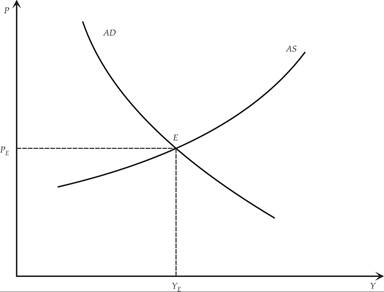
Figure 15.3 Aggregate output and the price level: the AD-AS model.

To derive the aggregate supply function AS, we examine the behavior of the representative firm. Assume that the representative firm is competitive and maximizes profits, selecting the level of employment and output, and taking nominal wages and prices as given. Output and employment are determined by solving the following optimization problem:

under the constraint

where F is a concave short-run production function, depending only on the level of employment L.

The maximization leads to a downward-sloping labor demand curve with respect to the real wage. Thus, employment is determined by the condition

Because the marginal product of labor is a negative function of the level of employment, the demand for labor is negatively related to the real wage W/P.

Solving (15.11) for employment, and substituting in the production function (15.10), we get an aggregate supply function that is a negative function of the real wage. If the nominal wage is exogenously fixed (as assumed in this version of the Keynesian model), then aggregate supply is a positive function of the price level, as a higher price level is associated with a lower real wage. We thus have

where for a given nominal wage W, it follows that .

The higher the level of prices is, the lower the real wage will be, with the result that firms demand more labor and produce more. The aggregate supply function (15.11) is the upward-sloping curve AS in figure 15.3. Short-run equilibrium is at point E.¹¹

15.1.4 The Impact of Aggregate Demand Policies

Equations (15.8) and (15.11) and figure 15.3 can be used to analyze economic fluctuations and the impact of macroeconomic policy on both output (employment) and the price level in the standard Keynesian model.¹²

First, for given nominal wages, an economy can be trapped in a short-run equilibrium with high unemployment. Suppose that the entire workforce is equal to N. From the production function (15.10), full employment output and income is given by¹³

Consider figure 15.4. The original equilibrium is at full employment output. A negative disturbance in aggregate demand shifts the aggregate demand curve AD to the left. In the new short-run equilibrium E₁, income and employment decline, and the price level falls. Because of the rigidity of nominal wages, the economy moves to an equilibrium with lower real output and employment and positive unemployment.

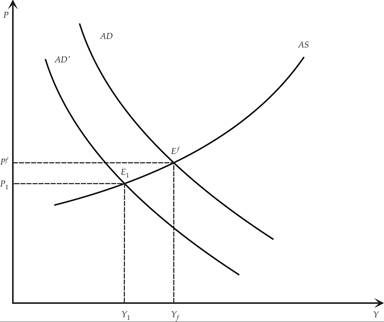
Figure 15.4 Aggregate demand disturbances and their effects on aggregate output and the price level.

If nominal wages were not fixed in the short run and adjusted to achieve full employment, the aggregate supply function would be perpendicular to the level of full employment, and changes in aggregate demand would only result in changes in the price level. Consequently, with full flexibility of wages and prices, this model has the same properties as a classical model.¹⁴

This model can also be used to address the effects of disturbances to aggregate supply. Consider figure 15.5. The original equilibrium is at full employment output. A negative disturbance in aggregate supply, such as a negative productivity shock, shifts the aggregate supply curve AS to the left. In the new short-run equilibrium, income and employment declines, and the price level rises. Because of the rigidity of nominal wages, the economy moves to an equilibrium with lower real output and employment, a higher price level, and positive unemployment.¹⁵

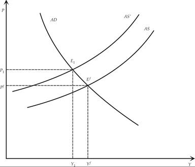
Figure 15.5 Aggregate supply disturbances and their effects on aggregate output and the price level.

In contrast to the classical model of full adjustment of wages and prices, in the Keynesian model with nominal wage rigidity, even monetary disturbances can shift aggregate demand and cause fluctuations in real output, employment, and other real variables (such as real wages and interest rates).

How can the impact of shocks to aggregate demand and supply be addressed? According to the Keynesian approach, an appropriate solution can come from macroeconomic policy. An increase of government expenditure, a reduction in taxes, or an increase in the money supply can move the aggregate demand curve to the right and counteract the consequences of a negative demand or supply shock, on real output and unemployment. In the case of demand shocks, the price level returns to its original equilibrium. In the case of a negative supply shock, there are further upward effects on the price level, so a trade-off occurs between unemployment and price stability. Thus, supply shocks cannot be effectively neutralized through aggregate demand policies, as trying to counteract them through aggregate demand policies has implications for the price level. In the case of a positive demand or supply shock, the opposite would apply.

We shall return to the question of role of aggregate demand policies in Keynesian models after we examine the Samuelson [1939] multiplier accelerator model, which is a dynamic version of the model of the Keynesian cross.

15.2