MODELING PORTFOLIO PERFORMANCE
The performance of the constructed portfolio is measured based on income simulation and expected liquidity. These have to be evaluated under both canonical expected conditions and stress scenarios.
13.4.1 Income performance
To estimate the return on investment of the portfolios, we need to estimate the performance of the sample portfolios under canonical conditions. Such conditions imply that all borrowers fulfill the agreed obligations. In an ideal world, the default probability is zero because none of the obligors will default. They will execute all principal and interest cash flow events as agreed without late payments, and they will also refrain from early payments, so the prepayment rate equals zero.
The return performance is based on a simple typical return of investment estimation, i.e., the net profit over the initial investment. Thus, the distribution of contract returns of a single
Exposure Profiles of Portfolio No 1 (Scenario Canonical)
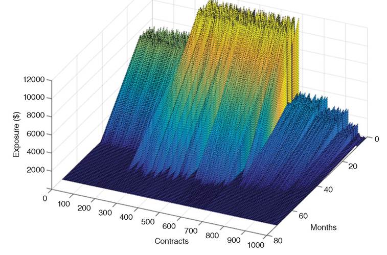
FIGURE 13.3 Portfolio exposure for scenario under canonical expectations
sample portfolio is as illustrated in Figure 13.4. Figure 13.5 shows the distribution of the returns referring to 1,000 sample portfolios.
These returns look good. The median total return of our sample portfolios is 23.9 percent during the overall duration14 of the contracts. The lower bound is 23.31 percent and the upper bound is 24.54 percent. The annual mean arithmetic return is 6.62 percent. Table 13.1 at the beginning of this chapter shows additional summary statistics of the different scenarios.
Let’s remember that this is the return under canonical conditions, where the market and all borrowers behave in exemplary fashion and get an A+ for their behavior.
13.4.2 Liquidity performance
In regards to liquidity, every single contract results in expected principal and interest cash flow payments.
As the portfolios in marketplace lending are not tradable, only funding liquidity is of interest in our analysis. In such analysis two types of liquidity reports are rather important: marginal and cumulative. Marginal liquidity focuses mainly on the view of in and out flows through time. Cumulative liquidity illustrates the evolution of the cash flows, where the investor can see the growth or deterioration of the expected cash in and out flows. Examples of these types of reports are illustrated in Figure 13.6 where marginal and cumulative liquidity GAP reports based on aggregated cash flows for portfolio number 1 under canonical conditions are shown; moreover, detailed evolution, of individual contracts of the portfolio, is illustrated in Figure 13.7.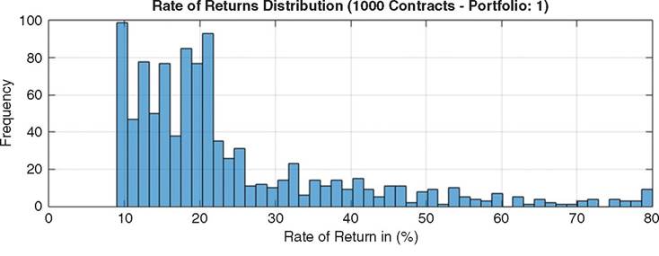
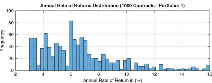
FIGURE 13.4 Rate of return distribution of a single sample portfolio during the entire duration of the investment
Moreover, Figure 13.8 illustrates the evolution of expected liquidity gaps of the entire distribution of 1,000 portfolios. When contracts mature, their cash flows become flat. Still, investors hold them until the last contract has matured.
Under normal conditions, we can say that “returns are quite good as long as the music plays.” Let's now investigate this claim by stressing the portfolios.
13.4.3 Stress testing
Under stress, portfolios perform differently from what we expect under canonical conditions. To simulate this, we stress the ratings, time of default, prepayments rate, and the point in time of the prepayments. We define these parameters based on the scenarios.
We assume that higher rated borrowers default less often than lower rated counterparties. When they do, defaults are expected to happen late. At the same time, they prepay more often than lower rated counterparties. When they do, they do so early.
The point in time where the default or prepayment occurs is defined as a percentage in regards to the duration of the contract; for instance an event (default or prepayment) at point in time 90 percent means that if a contract lasts 60 months, the default happens in month 54.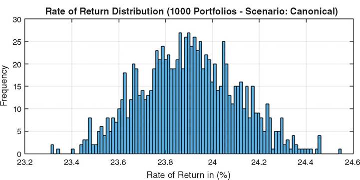
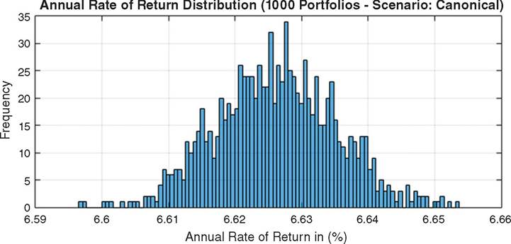
FIGURE 13.5 Distribution of the rate of returns under canonical conditions among all 1,000 sample portfolios
As aforementioned, and discussed in Chapter 7, we derive the default probabilities through annual time iterations, by using the hazard rate function defined in Equation 13.1, which is driven by the credit spread and recovery15 rates. The market risk-free fixed rates are set to 1.5%; to capture any volatility of this rate we apply an add-on random factor that may increase the above rate up to 2.5%. The remaining degree from the interest rate set in each contract defines the credit spread.
Obviously, a borrower with a higher rating pays a lower interest than a borrower with a lower rating, where the rating is the sum of market interest and the credit spread. Because these are all unsecured—uncollateralized—loans, nothing can compensate lenders in case of a default. We have therefore used the accumulated interest income that lenders receive as de-facto collateral or recovery just after the default against which we compile losses that occur in the event of a default. With this in mind, what is worse under these circumstances: defaults
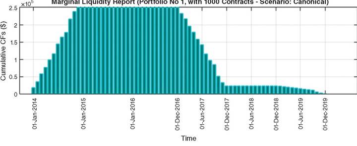
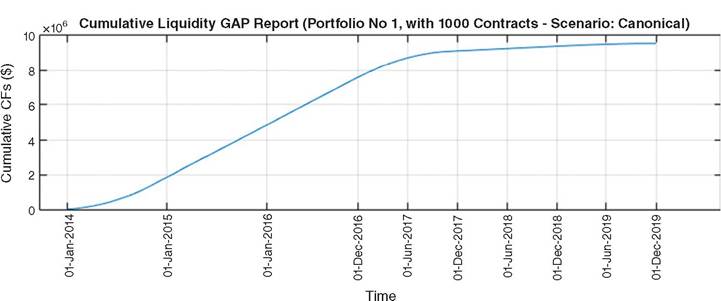
FIGURE 13.6 Marginal and cumulative liquidity GAP reports based on aggregated cash flows for portfolio No 1 resulted under canonical conditions
of higher rated borrowers or lower rated borrowers? Both result in losses, but because the higher rated borrowers pay much less interest than lower rated counterparties, their de-facto collateral is much smaller.
When they default, they can wipe out the accumulated interest over the period, quickly racking up losses. Investing in only the higher grades is therefore a bad risk mitigation strategy because defaults eat up the lower interest almost immediately. As a side note, Table 13.3 shows the interest rates that lenders can expect from each loan grade.16We used the default probability to estimate losses from cancelled interest and principal cash flows, after the point in time of default.
We stress the risk factor of credit spreads by applying deterministic shock that ranges based on the rating scale, i.e., from A1 to G5. Default rates for the two scenarios are described in the next paragraphs. Notably, the point in time of default plays a key role in the estimation of returns and losses.
Let's move on to prepayments. Market conditions affect both default and prepayments. The latter impact investors' interest income and the liquidity of the portfolio. Moreover, they impact the net exposure because we use interest income as collateral/recovery to cover losses. Prepayments therefore have an effect on the size of losses in case of defaults.
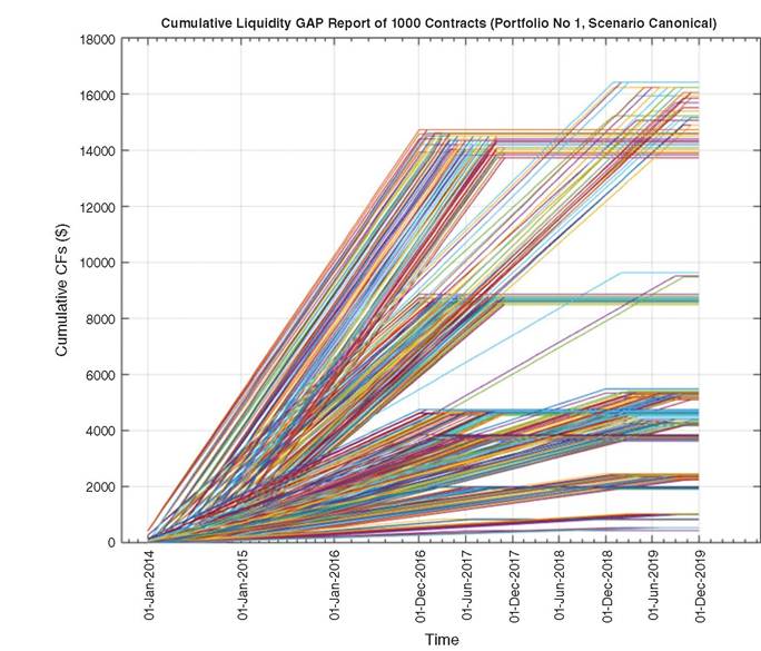
FIGURE 13.7 Cumulative liquidity GAP reports for each of the 1,000 contracts in portfolio number 1 under canonical conditions
13.4.4 Stresstestscenarios
As we discussed in Chapter 6, the main market risk factors are currencies, asset prices, yield curve and market interest rates, and product interest rates. Marketplace loans only have indirect exposure to market conditions; these also drive the probability of default and prepayments. Roughly speaking, in marketplace lending, all possible scenarios impact the same two things, either positively or negatively: default probability and prepayments. Let's now look at three different scenarios, summarized in Table 13.4.
13.4.4.1 Baseline case: Canonical conditions in the ideal world This is the outcome we all would like to see with our investments where they perform as expected.
We hardly need to describe this in more detail, as we have already looked at its results at the beginning of this chapter.Scenario A: Shock in the economy If the economy in general is under pressure with interest rates at low or negative levels, credit from formal channels may remain inaccessible for most counterparties. The market has little faith in counterparties to improve their economic prospects in the future, which would allow them to meet their obligations as borrowers. Stress in the market implies liquidity problems and insecurity. All parties in the economy have a
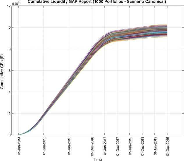
FIGURE 13.8 Distribution of cumulative liquidity GAP reports out of 1,000 portfolios
difficult time; some people may lose their jobs, and those who run a business will have to brace themselves for rough weather ahead. Borrowers of marketplace loans pay high fixed interest rates for a relatively long duration of three to six years. They may have signed up for a high rate loan because they were hoping for a market upswing. Being stuck with such a loan is especially severe for small businesses. They may have borrowed to improve their business prospects, but in an economic slump, customers fail to materialize. The longer that very low
TABLE 13.3 Interest rate and ARP Lending Club
| Loan grade | Annual interest rate | Origination fee | 36-Month APR | 60-Month APR |
| A | 5.32%-7.98% | 1%-4% | 5.99%-9.97% | 7.02%-9.63% |
| B | 8.18%-11.53% | 4%-5% | 10.98%-14.38% | 10.38%-13.80% |
| C | 12.29%-14.65% | 5% | 15.90%-18.31% | 14.58%-16.99% |
| D | 15.61%-17.86% | 5% | 19.29%-21.60% | 17.98%-20.28% |
| E | 18.25%-20.99% | 5% | 21.99%-24.80% | 20.68%-23.49% |
| F | 21.99%-25.78% | 5% | 25.82%-29.70% | 24.51%-28.40% |
| G | 26.77%-28.99% | 5% | 30.71%-32.99% | 29.42%-31.70% |
Data source: Lending Club, as of May 21, 2015
| TABLE 13.4 | Stress test scenarios and their simulation | ||
| Canonical conditions | Scenario A | Scenario B | |
| Description | Nothing changes | Shock in the economy, the | Shock in the economy |
| whole market | with extra stress on | ||
| underperforms | alternative borrowers | ||
| Assumptions | Prepayments → | Prepayments / | Prepayments / |
| Defaults → | Defaults ↑ | Defaults ↑ | |
| Simulation | No change of expected | Stress on counterparty | Stress on counterparty |
| defaults and prepayments | spreads and prepayments | spreads and prepayments | |
interest rates persist—a sign that the economy is doing badly—the higher the likelihood of a behavior change in borrowers. We must assume that market conditions change eventually, that they will not stay the same.
With this in mind, it becomes apparent that fixed interest rates are riskier than we expected. In the long run, nothing stays the same. When market conditions change, borrowers may choose to default because they simply lack the funds to pay back the loan. People have fewer options to make more money, and the default probability is increasing. On the flipside, few highly rated counterparties prepay their existing loans because they simply lack the funds to do so. We simulate this scenario by stressing the counterparty spreads across all grades and decreasing the frequency of prepayments marginally.Scenario B: Shock in the economy with extra stress on alternative borrowers When the economy tanks, it often affects all people in one form or another. This is roughly what Scenario A is all about. In Scenario B, we put added stress on borrowers relying on credit outside the formal financial system. Defaults in the sector may occur for several reasons. For example, platforms may have a hard time underwriting marketplace loans. Reasons for this may be that their cost of capital has gone up through time, or that regulation has stepped up the rules, which have made it more difficult to service middle to low-rated borrowers. If marketplace lending runs into liquidity problems at the same time that the economy is under shock, a vicious cycle begins: borrowers come under stress as they see that the alternative credit system, their lifeline for capital, is at risk. Shouldered with high fixed interest rate and a relatively long maturity, borrowers may default. As a result, their credit scores suffer and they become even less eligible for credit. As a group, marketplace borrowers might act similarly in economic turmoil. Lowerrated loans have a high default probability and credit spread, so their defaults in times of stress are less of a surprise. Conversely, when high-rated counterparties default—those that we assumed would be secure—it takes investors by surprise. How prepayments behave in this scenario is unclear. They may remain steady but most likely they will be reduced due to liquidity problems. A higher frequency of prepayments on the other hand may be the case if competitors decide to take advantage of the weakness of those platforms that are under the heaviest scrutiny by offering lower rates that allow borrowers to prepay; however they will rather look for the higher rated counterparties. Higher rated counterparties may therefore prepay to restructure their portfolios. Sources of stress for platforms are manifold. Another possible cause for distress for the sector might be that lenders lose the appetite to invest in their loans. We simulate this scenario with a higher rate of default and a high frequency of prepayments, expected from highly rated borrowers.
13.4.4.2 Simulating scenarios Wesimulateourscenariosbystressingthreevariables: the risk factor of the credit spreads, the times of default, and the probabilities of prepayment rates and the time of prepayment. The following paragraphs explain each variable.
Stressing risk factor of credit spreads Spreads have been shocked17 based on the underlying counterparty rating in contracts. The default probabilities, starting with initial spreads linked to rating classes, are changing over time based on hazard rates. The new default rates range from 8% for rating A1 to 99% for rating G5. This actually defines the shocks of the ratings, which will immediately affect credit spreads. For instance, within the duration of the contracts, in Scenario A the spread for counterparties rate A1 may rise, but only 0.1%. However, in Scenario B, the spread for the lowest rated counterparties may rise by up to 99%.
Stressing times of default Default events occur at an expected point in time, depending on a contract’s counterparty rating.18 We expect contracts with high ratings to default later in the term, and contracts with low ratings earlier. In Scenario A, counterparties rated A1 default at or after 84% of the life of the contract, while contracts rated G5 default at or after 20% of their life. For instance, a contract maturing in 36 months with a default time of 84% is expected to default after 30.2 months. Figure 13.9 and Figure 13.10 illustrate the default rates and times applied to all 1,000 contracts in the analysis according to their sub-grades A1 to G5. To make the simulation more pragmatic, we increase the volatility of the rates and times by adding a small noise factor between zero and ten percent.
Default rates and times shown in Figure 13.9 were aligned with Scenario A where lower rated counterparties are expected to default. The first 690 contracts (rated A1 to B5) have defaulted with a rate from 6% to 36%. As expected, the PITs of such defaults appear late— from 72% to 84% of the duration of the contracts. The 310 remaining contracts default with a rate from 40% to 100% at the PITs from 36% to 71% of the life of the contracts. On the other hand, in Scenario B (Figure 13.10), the default rate increases for the contracts with median ratings B and C. The first 690 contracts with A1 to B5 ratings have a default rate of less than 48%, and these defaults occur late. The remaining contracts default from 49% to 100% at the PITs from 20% to 49% of the contracts’ life.
Stressing probabilities of prepayment rates and the time of prepayment The top prepayment rate is 25.5% for Scenario A and 60% for Scenario B. The time of each prepayment is set as a percentage of the contract’s duration. Figure 13.11 and Figure 13.12 show the amount and times of prepayments for each contract. In Scenario A, the PITs of prepayments range from medium to late—35% to 99% of the life of the contract. In Scenario B, prepayments are higher. The first 690 contracts, rated A1 to B5, will prepay 46% to 60% of their principal during the first third of their duration. The remaining contracts will be also prepay, but will prepay smaller amounts, and later in the life of the contract.
13.4.4.3 Outcomes Based on the above scenarios the system calculated all financial events for the 1,000 contracts of the 1,000 portfolios. As we mentioned earlier, the return performance is based on a simple typical return of investment estimation. The distributions of the returns for the 1,000 sample portfolios, based on Scenarios A and B, are illustrated in Figure 13.13 and Figure 13.14 respectively.
In Scenario A, the median total return of our sample portfolios is 4.02% during the overall duration of the contracts. The lower bound is 3.9% and the upper bound is 4.12%. The annual
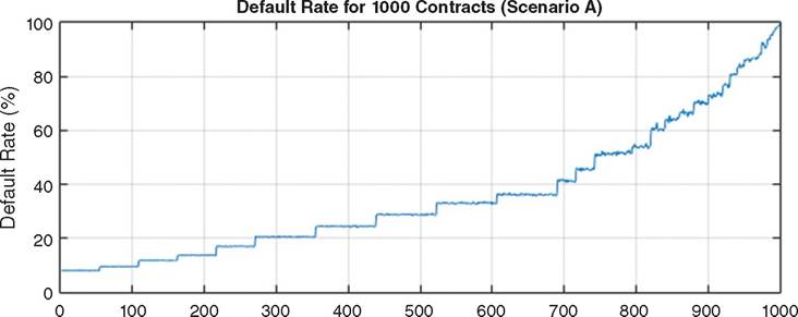
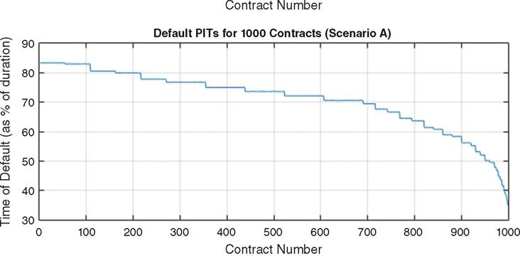
FIGURE 13.9 Default rate (in percentage) and the time of default as percentage of individual contracts’ duration applied, for Scenario A, to each group, classified from A1 to G5 ratings, of the 1,000 contracts constructing the simulated portfolios
mean arithmetic return is 1.42%. Returns for Scenario A are still positive but rather close to what an investor could get from the established financial institutions which also provide 100% guarantee of returning the full amount of the capital.
In Scenario B, the median total return during the overall duration of the contracts, reaches a negative return on investment of -18.3%, with the lower and higher bounds estimated at -18.68% and -17.94% respectively. Moreover, the annual mean return is -5.1%. In this case, investors are suffering losses that the interest income cannot cover.
The distribution of cumulative liquidity GAP reports out of 1,000 portfolios for both Scenario A and Scenario B are illustrated in Figure 13.15 and Figure 13.16. As we can see, the cumulative cash flows have been reduced 24.8%.
From Figure 13.17 and Figure 13.18 we can observe that the evolution of the contracts’ net exposures have increased over time. This is because due to stress scenarios the interest income, which is considered as the amount to collateralize the gross exposure, has decreased;
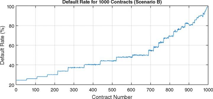
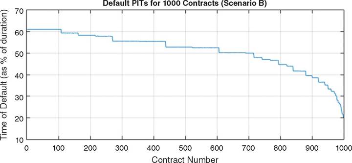
FIGURE 13.10 Default rate in percentage and the time of default as percentage of individual contracts’ duration applied, for Scenario B, to each group, classified from A1 to G5 ratings, of the 1,000 contracts constructing the simulated portfolios
thus, the net exposure has been increased accordingly. Figure 13.19 illustrates the evolution of the portfolio exposures under the three scenarios (i.e., Canonical, A and B).
13.5