The Mathematical Theory of Probability
In probability theory, we see two types of probabilities: absolute probabilities and conditional probabilities. Absolute probabilities (also known as unconditional probabilities) are probabilities of the form “P(A)” while conditional probabilities are probabilities of the form “P(A, B)” - read as “the probability of A, given B.”[55] These two types of probability can be defined in terms of each other.
So when formalizing the notion of probability we have a choice: do we define conditional probability in terms of unconditional probability, or vice versa? The next section, §2.1, will focus on some of the various formal theories of probability that take absolute probability as primitive and define conditional probability in terms of the former. Then in §2.2, we will look at some of the various formal theories that take conditional probability as the primitive type of probability.2.1 Absolute probability as primitive
Kolmogorov’s theory of probability (Kolmogorov 1933) is the best known formal theory of probability and it is what you will learn if you take a course on probability. First, we start with a set of elementary events, which we will refer to by Q. For example, if we are considering the roll of a die where the possible outcomes are the die landing with “one” face up, or with “two” face up, etc., then Q would be the set {1, 2, 3, 4, 5, 6}. From this set of elementary events, we can construct other, less fine-grained events. For example, there is the event that an odd number comes up. We represent this event with the set {1, 3, 5}. Or, there is the event that some number greater than two comes up. We represent this event with set {3, 4, 5, 6}. In general, any event constructed from the elementary events will be a subset of Q. The least fine-grained event is the event that something happens - this event is represented by Q itself.
There is also the event that cannot happen, which is represented by the empty set, 0.[56]In probability theory, we often want to work with the set of all events that can be constructed from Q. In our die example, this is because we may want to speak of the probability of any particular number coming up, or of an even or odd number coming up, of a multiple of three, a prime number, etc. It is typical to refer to this set by F. In our example, if F contains every event that can be constructed from Q, then it would be rather large. A partial listing of its elements would be: F = {0, Q, {1}, {2}... {6}, {1, 2, 3}, {4, 5, 6}, {1, 2}, {1, 2, 3, 4, 5}...}. In fact, there are a total of 26 = 64 elements in F.
In general, if an event, A, is in F, then so is its complement, which we write as Q \ A. For example, if {3, 5, 6}, is in F, then its complement Q \ {3, 5, 6} = {1, 2, 4} is in F. Also, if any two events are in F, then so is their union. For example, if {1, 2} and {4, 6} are in F, then their union {1, 2} U {4, 6} = {1, 2, 4, 6} is in F. If a set, S, has the first property (i.e., if A is in S, then Q \ A is in S), then we say S is closed under Q-complementation. If S has the second property (i.e., if A and B are in S, then A U B is in S), then we say S is closed under union. And if S has both of these properties, i.e., if it is closed under both Q-complementation and union, then we say that S is an algebra on Q. If a set, S, is an algebra, then it follows that it is also closed under intersection, i.e., that if A and B are in S, then A P B is also in S.
In our die example, it can be seen that F (the set that contains all the subsets of Q) is an algebra on Q. However, there are also algebras on Q that do not contain every event that can be constructed from Q. For example, consider the following set: F = {0, {1, 3, 5}, {2, 4, 6}, Q}. The elements of this F would correspond to the events: (i) nothing happens; (ii) an odd number comes up; (iii) an even number comes up; and (iv) some number comes up.
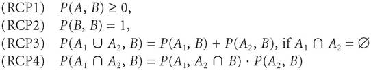
This is an important example of an algebra because it illustrates how algebras work. For example, not every “event” - intuitively understood - gets a probability. For instance, the event that the number two comes up gets no probability because {2} is not in F. Also note that even though this F does not contain every subset of Q, it is still closed under union and Q-complementation. For example, the union of {1, 3, 5} and {2, 4, 6} is Q, which is in F, and the Q-complement of, say, {1, 3, 5} is {2, 4, 6}, which is also clearly in F.Once we have specified an algebra, F, we can then define a probability function that attaches probabilities to every element of F. Let P be a function from F to the real numbers, R, that obeys the following axioms:
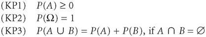
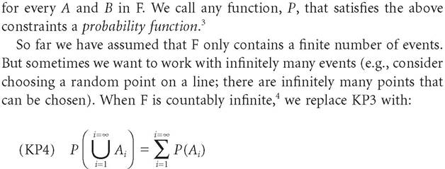
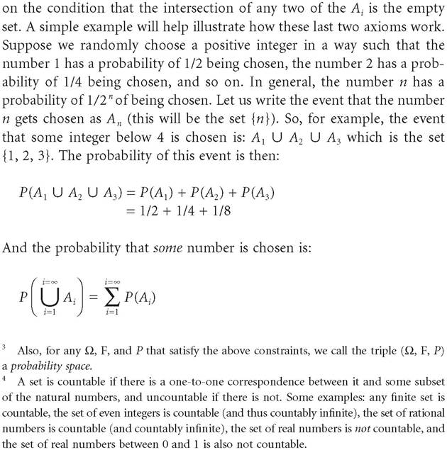
which can be expanded as:
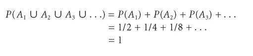
This fourth axiom - known as countable additivity - is by far the most controversial. Bruno de Finetti (1974) famously used the following example as an objection to KP4. Suppose you have entered a fair lottery that has a countably infinite number of tickets. Since the lottery is fair, each ticket has an equal probability of being the winning ticket. But there are only two ways in which the tickets have equal probabilities of winning, and on both ways we run into trouble. On the first way, each ticket has some positive probability of winning - call this positive probability £. But then, by KP4, the probability that some ticket wins is £ added to itself infinitely many times, which equals infinity, and so violates KP2. The only other way that the tickets can have equal probability of winning is if they all have zero probability.
But then KP4 entails that the probability that some ticket wins is 0 added to itself infinitely many times, which is equal to zero and so again KP2 is violated. It is a matter of either too much or too little!Axioms KP1-4 define absolute probability functions on sets. However, many philosophers and logicians prefer to define probability functions on statements, or even other abstract objects instead. One reason for this is because Kolmogorov’s axioms are incompatible with many philosophical interpretations of probability. For example, Karl Popper points out that the formal theory of probability should be sensitive to the needs of the philosophical theory of probability:
In Kolmogorov’s approach it is assumed that the objects a and b in p(a, b) are sets (or aggregates). But this assumption is not shared by all interpretations: some interpret a and b as states of affairs, or as properties, or as events, or as statements, or as sentences. In view of this fact, I felt that in a formal development, no assumption concerning the nature of the “objects” or “elements” a and b should be made [...]. (Popper 1959b, 40)
A typical alternative to Kolmogorov’s set-theoretic approach to probability is an axiom system where the bearers of probability are sentences (in §2.2,
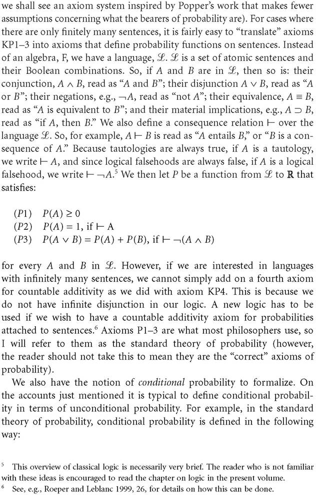
Many have pointed out that this definition leaves an important class of conditional probabilities undefined when they should be defined. This class is comprised of those conditional probabilities of the form, P(A, B) where P (B) = 0. Consider the following example, due to Emile Borel.[57] Suppose a point on the earth is chosen randomly - assume the earth is a perfect sphere. What is the probability that the point chosen is in the western hemisphere, given that it lies on the equator? The answer intuitively ought to be 1/2.
However, CP does not deliver this result, because the denominator - the probability that the point lies on the equator - is zero.[58]There are many responses one can give to such a problem. For instance, some insist that any event that has a probability of zero cannot happen. So the probability that the point is on the equator must be greater than zero, and so CP is not undefined. The problem though is that it can be proven that for any probability space with uncountably many events, uncountably many of these events must be assigned zero probability, as otherwise we would have a violation of the probability axioms.[59] This proof relies on particular properties of the real number system, R. So some philosophers have said so much the worse for the real number system, opting to use a probability theory where the values of probabilities are not real numbers, but rather something more mathematically rich, like the hyperreals, HR (see, e.g., Lewis 1980, Skyrms 1980).[60]
Another response that philosophers have made to Borel's problem is to opt for a formal theory that takes conditional probability as the fundamental notion of probability (we will see some of these theories in §2.2). The idea is that by defining absolute probability in terms of conditional probability while taking the latter as the primitive probability notion to be axiomatized, conditional probabilities of the form P(A, B) where P(B) = 0 can be defined.[61]
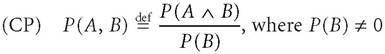
There are, also, other reasons to take conditional probability as the fundamental notion of probability. One such reason is that sometimes the unconditional probabilities P(A a B) and P(B) are undefined while the conditional probability P(A, B) is defined, so it is impossible to define the latter in terms of the former. The following is an example due to Alan Hajek (2003). Consider the conditional probability that heads comes up, given that I toss a coin fairly. Surely, this should be 1/2, but CP defines this conditional probability as:
But you have no information about how likely it is that I will toss the coin fairly.
For all you know, I never toss coins fairly, or perhaps I always toss them fairly. Without this information, the terms on the right-hand side of the above equality may be undefined, yet the conditional probability on the left is defined.There are other problems with taking absolute probability as the fundamental notion of probability (see Hajek 2003 for a discussion). These problems have led many authors to take conditional probability as primitive. However, this requires a new approach to the formal theory of probability. And so we now turn to theories of probability that take conditional probability as the primitive notion of probability.
2.2 Conditional probability as primitive
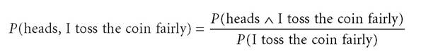
The following axiom system - based on the work of Alfred Renyi (1955) - is a formal theory of probability where conditional probability is the fundamental concept. Let Q be a non-empty set, A be an algebra on Q, and B be a nonempty subset of A. We then define a function, P, from A X B to R such that:[62]
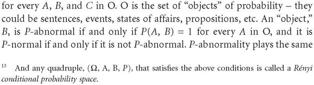
where the As are in A and the Bs are in B. Any function that satisfies these axioms is called a Renyi conditional probability function.13 RCP3 is the conditional analogue of the KP3 finite additivity axiom and it also has a countable version:
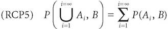
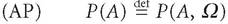
on the condition that the Ai are mutually exclusive. RCP4 is the conditional analogue of CP, and absolute probability can then be defined in the following way:
Popper, in many places, gives alternative axiomatizations of probability where conditional probability is the primitive notion (see, e.g., Popper 1938, 1955, 1959a, 1959b). The following set of axioms is a user-friendly version of Popper's axioms (these are adapted from Roeper and Leblanc 1999, 12):
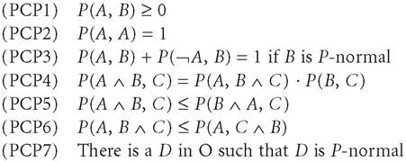
role as logical falsehood. Any function, P, that satisfies the above axioms is known as a Popper conditional probability function, or often just as a Popper function, for short. This axiom system differs from Renyi’s in that: (i) it is symmetric (i.e., if P(A, B) exists, then P(B, A) exists), and (ii) it is autonomous. An axiom system is autonomous if, in that system, probability conclusions can be derived only from probability premises. For example, the axiom system P1-3 is not autonomous, because, for instance, we can derive that P(A) = 1, from the premise that A is a logical truth.
2.2 Other formal theories of probability
We have just seen what may be the four most prominent formal theories of probability. But there are many other theories also on the market - too many to go into their full details here, so I will merely give a brief overview of the range of possibilities.
Typically it is assumed that the logic of the language that probabilities are defined over is classical logic. However, there are probability theories that are based on other logics. Brian Weatherson, for instance, introduces an intuitionistic theory of probability (Weatherson 2003). He argues that this probability theory, used as a theory of rational credences, is the best way to meet certain objections to Bayesianism (see §3.5.2). The defining feature of this formal account of probability is that it allows an agent to have credences in A and — A that do not sum to 1, but are still additive. This can be done because it is not a theorem in this formal theory of probability that P(A v —iA) = 1.
Another example of a “non-classical” probability theory is quantum probability. Quantum probability is based on a non-distributive logic, so it is not a theorem that P((A a B) v C) = P((A v C) a (B v C)). Hilary Putnam uses this fact to argue that such a logic and probability makes quantum mechanics less mysterious than it is when classical logic and probability theory are used (Putnam 1968). One of his examples is how the incorrect classical probability result for the famous two-slit experiment does not go through in quantum probability (see Putnam 1968 for more details and examples). See Dickson (2001) - who argues that quantum logic (and probability) is still a live option for making sense of quantum mechanics - for more details and references.
As we will see in §3.5, the probability calculus is often taken to be a set of rationality constraints on the credences (degrees of belief) of an individual. A consequence of this - that many philosophers find unappealing - is that an individual, to be rational, should be logically omniscient. Ian Hacking introduces a set of probability axioms that relax the demand that an agent be logically omniscient (Hacking 1967).
Other formal theories of probability vary from probability values being negative numbers (see, e.g., Feynman 1987), to imaginary numbers (see, e.g., Cox 1955), to unbounded real numbers (see, e.g., Renyi 1970), to real numbered intervals (see, e.g., Levi 1980). Dempster-Shafer Theory is also often said to be a competing formal theory of probability (see, e.g., Shafer 1976). For more discussion of other formal theories of probability, see Fine (1973).
That concludes our survey of the various formal theories of probability. So far, though, we have only half of the picture. We do not yet have any account of what probabilities are, only how they behave. This is important because there are many things in the world that behave like probabilities, but are not probabilities. Take, for example, areas of various regions of a tabletop where one unit of area is the entire area of the tabletop. The areas of such regions satisfy, for example, Kolmogorov’s axioms, but are clearly not probabilities.
3.