The Philosophical Theory of Probability

Interpretations of probability are typically categorized into two kinds: subjective interpretations and objective interpretations. Roughly, the dif­ference is that subjective interpretations identify probabilities with the credences, or “degrees of belief,” of a particular individual, while objective interpretations identify probability with something that is independent of any individual - the most common somethings being relative frequencies and propensities.

3.1 The classical interpretation

The central idea behind the classical interpretation of probability - historically the first of all the interpretations - is that the probability of an event is the ratio between the number of equally possible outcomes in which the event occurs and the total number of equally possible outcomes. This concep­tion of probability is particularly well suited for probability statements concerning games of chance. Take, for example, a fair roll of a fair die. We quite naturally say that the probability of an even number coming up is 3/6 (which, of course, is equal to 1/2). The “3” is for the three ways in which an even number comes up (2, 4, and 6) and the “6” is for all of the possible numbers that could come up (1, 2, 3, 4, 5, and 6).

The idea of relating probabilities to equally possible outcomes can be found in the works of many great authors - e.g., Cardano (1663), Laplace (1814) and Keynes (1921). However, among these authors there is a considerable degree of variation in how this idea is fleshed out. In particular, they vary on how we are to understand what it means for events to be “equally possible.” In the hands of some, the equally possible outcomes are those outcomes that are symmetric in some physical way.

The theory of chance consists in reducing all the events of the same kind to a certain number of cases equally possible, that is to say, to such as we may be equally undecided about in regard to their existence, and in determining the number of cases favorable to the event whose probability is sought. (Laplace 1814, 6; emphasis added)

Understood this way, the classical interpretation is a subjective interpret­ation of probability. From now on, I will assume that the classical interpreta­tion is a subjective interpretation, as this is the most popular understanding of the interpretation - see Hacking (1971) for a historical study of the notion of equal possibilities and the ambiguities in the classical interpretation.

If we follow Laplace, then the classical interpretation puts constraints on how we ought to assign probabilities to events. More specifically, it says we ought to assign equal probability to events that we are “equally un­decided about.” This norm was formulated as a principle now known as the Principle of Indifference by John Maynard Keynes:

If there is no known reason for predicating of our subject one rather than another of several alternatives, then relative to such knowledge the assertions of each of these alternatives have an equal probability. (Keynes 1921, 42) It is well known that the Principle of Indifference is fraught with paradoxes - many of which originate with Joseph Bertrand (1888). Some of these paradoxes are rather mathematically complicated, but the following is a simple one due to Bas van Fraassen (1989).

There have been several attempts to save the classical interpretation and the Principle of Indifference from paradoxes like the one above, but many authors consider the paradoxes to be decisive. See Keynes (1921) and van Fraassen (1989) for a detailed discussion of the various paradoxes, and see Jaynes (1973), Marinoff (1994), and Mikkelson (2004) for a defense of the principle. Also see Shackel (2007) for a contemporary overview of the debate. The existence of paradoxes like the one above was one source of motiva­tion for many authors to abandon the classical interpretation and adopt the frequency interpretation of probability.

3.2 The frequency interpretation

3.2.1 Actual frequencies

Ask any random scientist or mathematician what the definition of prob­ability is and they will probably respond to you with an incredulous stare or, after they have regained their composure, with some version of the frequency interpretation.

But which people are like John? If we consider all those Englishmen aged 50, then we will include consumptive Englishmen aged 50 and all the healthy ones too. Intuitively, the fact that John is sickly should mean we only consider consumptive Englishmen aged 50, but where do we draw the line? Should we restrict the class of those people we consider to those who are also named John? Surely not, but is there a principled way to draw the line? If there is, it is hard to say exactly what that principle is. This is important because where we draw the line affects the value of the probability. This problem is known as the reference class problem. John Venn was one of the first to notice it:

It is obvious that every individual thing or event has an indefinite number of properties or attributes observable in it, and might therefore be considered as belonging to an indefinite number of different classes of things [...]. (Venn 1876, 194)

This can have quite serious consequences when we use probability in our decision making (see, e.g., Colyvan, Regan, and Ferson 2001). Many have taken the reference class problem to be a difficulty for the frequency inter­pretation, though Mark Colyvan et al.

The frequency interpretation is like the classical interpretation in that it identifies the probability of an event with the ratio of favorable cases to cases. However, it is unlike the classical interpretation in that the cases have to be actual cases. Unfortunately, this means that the interpretation is shackled too tightly to how the world turns out to be. If it just happens that I never flip this coin, then the probability of “tails” is undefined. Or if it is flipped only once and it lands “tails,” then the probability of “heads” is 1 (this is known as a single case probability). To get around these difficul­ties many move from defining probability in terms of actual frequencies to defining it in terms of hypothetical frequencies. There are many other problems with defining probability in terms of actual frequencies (see Hajek 1997 for 15 objections to the idea), but we now move on to hypothetical frequencies.

3.2.2 Hypothetical frequencies

The hypothetical frequency interpretation tries to put some of the modality back into probability. It says that the probability of an event is the number of trials in which the event occurs divided by the number of trials, if the trials were to occur. On this frequency interpretation, the trials do not have to actually happen for the probability to be defined. So for the coin that I never flipped, the hypothetical frequentist can say that the probability of “tails” is 1/2 because this is the frequency we would observe, if the coin were tossed.

Maybe. But we definitely would not observe this frequency if the coin were flipped an odd number of times, for then it would be impossible to observe an even number of “heads” and “tails” events. To get around this sort of problem, it is typically assumed that the number of trials is count­ably infinite, so the frequency is a limiting frequency. Defenders of this type of view include Richard von Mises (1957) and Hans Reichenbach (1949).

THTTHTHHT...

where T is for “tails” and H is for “heads.” We calculate the limiting fre­quency by calculating the frequencies of successively increasing finite sub­sequences. So for example, the first subsequence is just T, so the frequency of “tails” is 1. The next larger subsequence is TH, which gives a frequency of 1/2. Then the next subsequence is THT, so the frequency becomes 2/3. Continuing on in this fashion:

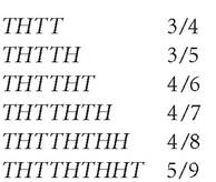
These frequencies appear to be settling down to the value of 1/2. If this is the case, we say that the limiting frequency is 1/2. However, the value of the limiting frequency depends on how we order the trials. If we change the order of the trials, then we change the limiting frequency. To take a simple example, consider the following sequence of natural numbers: (1, 2, 3, 4, 5, 6, 7, 8, 9, 10, 11,...). The limiting frequency of even numbers is 1/2. Now consider a different sequence that also has all of the natural numbers as elements, but in a different order: (1, 3, 5, 2, 7, 9, 11, 4,...). Now the limiting frequency of even numbers is 1/4. This means that the value of a limiting frequency is sensitive to how we order the trials, and so if prob­abilities are limiting frequencies, then probabilities depend on the order of the trials too. This is problematic because it seems probabilities should be independent of how we order the trials to calculate limiting frequencies.^[63]

Another worry with the hypothetical frequency interpretation is that it does not allow limiting frequencies to come apart from probabilities. Suppose a coin, whenever flipped, has a chance of 1/2 that “tails” comes up on any particular flip. Although highly improbable, it is entirely possible that “tails” never comes up. Yet the hypothetical frequency interpretation says that this statement of 50 percent chance of “tails” means that the limiting frequency of “tails” will be 1/2. So a chance of 1/2 just means that “tails” has to come up at least once (in fact, half of the time). Many philo­sophers find this unappealing, for it seems that it is part of the concept of probability that frequencies (both finite and limiting frequencies) can come apart from probabilities.

One of the motivations for the move from the actual frequency inter­pretation to the hypothetical frequency interpretation was the problem of single-case probabilities. This was the problem that the actual frequency interpretation cannot sensibly assign probabilities to one-time-only events. This problem was also a main motivation for another interpretation of probability, the propensity interpretation.

3.3 The propensity interpretation

The propensity interpretation of probability originates with Popper in Popper 1957, and was developed in more detail in Popper 1959b. His motivation for introducing this new interpretation was the need, that he saw, for a theory of probability that was objective, but that could also make sense of single-case probabilities - particularly the single-case probabilities which he thought were indispensable to quantum mechanics. His idea was (roughly) that a probability is not a frequency, but rather it is the tendency, the disposition, or the propensity of an outcome to occur.

Popper, who was originally a hypothetical frequentist, developed the propensity theory of probability as a slight modification of the frequency theory. The modification was that instead of probabilities being properties of sequences (viz., frequencies), they are rather properties of the condi­tions that generate those sequences, when the conditions are repeated: “This modification of the frequency interpretation leads almost inevitably to the conjecture that probabilities are dispositional properties of these conditions - that is to say, propensities” (Popper 1959b, 37). And earlier: “Now these propensities turn out to be propensities to realize singular events” (Popper 1959b, 28; author's emphasis).

Perhaps the best known and most influential objection to Popper's original propensity interpretation is due to Paul Humphreys, and is known as Humphreys' paradox - though Humphreys himself did not intend the objection to be one against the propensity interpretation (Humphreys 1985). The objection, in a nutshell, is that propensities are not symmetric, but according to the standard formal theory of probability, probabilities are.^[64] For example, it is often possible to work out the probability of a fire having been started by a cigarette given the smoking remains of a building, but it seems strange to say that the smoking remains have a propensity, or dis­position, for a cigarette to have started the fire. The standard reaction to this fact has been “if probabilities are symmetric and propensities are not, then too bad for the propensity interpretation.” Humphreys, however, intended his point to be an objection to the standard formal theory of prob­ability (Humphreys 1985, 557) and to the whole enterprise of interpret­ing probability in a way that takes the formal theory of probability as sacrosanct:

It is time, I believe, to give up the criterion of admissibility [the criterion that a philosophical theory of probability should satisfy “the” probability calculus]. We have seen that it places an unreasonable demand upon one plausible construal of propensities. Add to this the facts that limiting relative frequencies violate the axiom of countable additivity and that their probability spaces are not sigma-fields unless further constraints are added; that rational degrees of belief, according to some accounts, are not and can­not sensibly be required to be countably additive; and that there is serious doubt as to whether the traditional theory of probability is the correct account for use in quantum theory. Then the project of constraining semantics by syntax begins to look quite implausible in this area. (Humphreys 1985, 569-70)

In response to Humphreys’ paradox, some authors have offered new formal accounts of propensities. For example, James Fetzer and Donald Nute de­veloped a probabilistic causal calculus as a formal theory of propensities (see Fetzer 1981). A premise of the argument that leads to the paradox is that probabilities are symmetric. But as we saw in §2.2, there are formal theories of probability that are asymmetric - Renyi’s axioms for conditional probability, for instance. A proponent of Popper’s propensity interpretation could thus avoid the paradox by adopting an asymmetric formal theory of probability. Unfortunately for Popper, though, his own formal theory of probability is symmetric.

There are now many so-called propensity interpretations of probability that differ from Popper’s original account. Following Donald Gillies, we can divide these accounts into two kinds: long-run propensity inter­pretations and single-case propensity interpretations (Gillies 2000b). Long-run propensity interpretations treat propensities as tendencies for certain conditions to produce frequencies identical (at least approxi­mately) to the probabilities in a sequence of repetitions of those conditions. Single-case propensity interpretations treat propensities as dispositions to produce a certain result on a specific occasion. The propensity interpreta­tion initially developed by Popper (1957, 1959b) is both a long-run and single-case propensity interpretation. This is because Popper associates propensities with repeatable “generating conditions” to generate singular events. The propensity interpretations developed later by Popper (1990), and David Miller (1994, 1996), can be seen as only single-case propensity interpretations. These propensity interpretations attribute propensities not to repeatable conditions, but to entire states of the universe. One problem with this kind of propensity interpretation is that probability claims are no longer testable, a cost noted by Popper himself (1990, 17). This is because probabilities are now properties of entire states of the universe - events that are not repeatable - and Popper believed that to test a probability claim, the event needs to be repeatable so that a frequency can be measured.^[65]

For a general survey and classification of the various propensity theo­ries, see Gillies (2000b); and see Eagle (2004) for 21 objections to them.

3.4 Logical probability

In classical logic, if — B, then we say A entails B. In model-theoretic terms, this corresponds to every model in which A is true, B is true. The logical interpretation of probability is an attempt to generalize the notion of entailment to partial entailment. Keynes was one of the earliest to hit upon this idea:

Inasmuch as it is always assumed that we can sometimes judge directly that a conclusion follows from a premiss, it is no great extension of this assumption to suppose that we can sometimes recognize that a conclusion partially follows from, or stands in a relation of probability to a premiss. (Keynes 1921, 52)

On this interpretation “P(B, A) = x” means A entails B to degree x. This idea has been pursued by many philosophers - e.g., William Johnson (1921), Keynes (1921), though Rudolf Carnap gives by the far the most developed account of logical probability (e.g., Carnap 1950).

By generalizing the notion of entailment to partial entailment, some of these philosophers hoped that the logic of deduction could be generalized to a logic of induction. If we let c be a two-place function that represents the confirmation relation, then the hope was that:

c (B, A) = P(B, A)

For example, the observation of ten black ravens deductively entails that there are ten black ravens in the world, while the observation of five black ravens only partially entails, or confirms, that there are ten black ravens, and the observation of two black ravens confirms this hypothesis to a lesser degree.

One seemingly natural way to formalize the notion of partial entailment is by generalizing the model theory of full entailment. Instead of B being true in every model in which A is true, we relax this to there being some percentage of the models in which A is true. So “P(B, A) = x,” which is to say, “A partially entails B to degree x” is true, if the number of models where B and A are true, divided by the number of models where A is true, is equal to x.^[66] If we think of models as like “possible worlds,” or possible outcomes then this definition is the same as the classical definition of probability. We might suspect then that the logical interpretation shares some of the same difficulties (in particular, the language relativity of probability) that the classical interpretation has. Indeed, this is so (see, e.g., Gillies 2000a, 29-49).

Carnap maintains that c(B, A) = P(B, A), but investigates other ways to define the probability function, P. In contrast to the approach above, Carnap's way of defining P is purely syntactic. He starts with a language with predicates and constants, and from this language defines what are called state descriptions. A state description can be thought of as a maximally specific description of the world. For example, in a language with predicates F and G, and constants a and b, one state description is Fa a Fb a Gb a —. Ga. Any state description is equivalent to a conjunction of predications where every predicate or its negation is applied to every constant in the language. Carnap then tried to define the probability function, P, in terms of some measure, m, over all of the state descriptions. In Carnap 1950, he thought that such a measure was unique. Later on, in Carnap 1963, he thought there were many such measures. Unfortunately, every way Carnap tried to define P in terms of a measure over state descriptions failed for one reason or another (see, e.g., Hajek 2007b).

Nearly every philosopher now agrees that the logical interpretation of probability is fundamentally flawed. However, if they are correct, this does not entail that a formal account of inductive inference is not possible. Recent attempts at developing an account of inductive logic reject the sole use of conditional probability and instead measure the degree to which evidence E confirms hypothesis H by how much E affects the probability of H (see, e.g., Fitelson 2006). For example, one way to formalize the degree to which E supports or confirms H is by how much E raises the probability of H:

c (H, E) = P(H, E) - P(H)

This is one such measure among many.^[67] The function c, or some other function like it, may formally capture the notion of evidential impact that we have, but these functions are defined in terms of probabilities. So an important and natural question to ask is: what are these probabilities? Perhaps the most popular response is that these probabilities are subjective probabilities, i.e., the credences of an individual. According to this type of theory of confirmation (known as Bayesian confirmation theory), the degree to which some evidence confirms a hypothesis is relative to the epistemic state of an individual. So E may confirm H for one individual, but dis­confirm H for another. This moves us away from the strictly objective rela­tionship between evidence and hypothesis that the logical interpretation postulated, to a more subjective one.

3.5 The subjective interpretation

While the frequency and propensity interpretations see the various formal accounts of probability as theories of how frequencies and propensities behave, the subjective interpretation sees them as theories of how people's beliefs ought to behave. We can find this idea first published by Frank Ramsey (1931) and de Finetti (1931a, 1931b). The normativity of the “ought” is meant to be one of ideal epistemic rationality. So subjectivists traditionally claim that for one to be ideally epistemically rational, one's beliefs must conform to the standard probability calculus. Despite the intuitive appeal of this claim (which by the way is typically called probabilism), many have felt the need to provide some type of argument for it. Indeed, there is now a formidable literature on such arguments. Perhaps the most famous argument for probabilism is the Dutch Book Argument.

3.5.1 The Dutch Book Argument

A Dutch book is any collection of bets that collectively guarantee a sure mon­etary loss. An example will help illustrate the idea. Suppose Bob assigns a credence of 0.6 to a statement, A, and a credence of 0.5 to that statement's negation, — A. Bob's credences thus do not satisfy the probability calculus since his credence in A and his credence in — A sum to 1.1. Suppose further that Bob bets in accordance with his credences, that is, if he assigns a credence of x to A, then he will buy a bet that pays $y if A, for at most $xy. Now consider the following two bets:

18

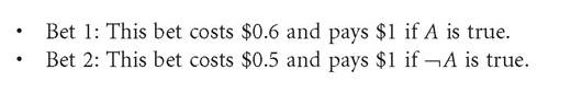
Bob evaluates both of these bets as fair, since the expected return - by his lights - of each bet is the price of that bet.^[68] But suppose Bob bought both of these bets. This would be apparently equivalent to him buying the following bet:

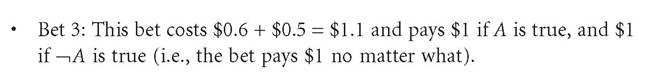
If Bob were to accept Bet 3, then Bob would be guaranteed to lose $0.1, no matter what. The problem for Bob is that he evaluates Bet 1 and Bet 2 as both individually fair, but by purchasing both Bet 1 and Bet 2, Bob effectively buys Bet 3, which he does not evaluate as fair (since his expected return on the bet is less than the price of the bet).

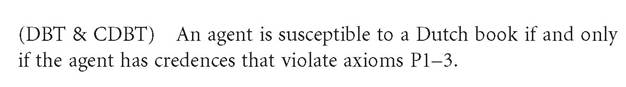
There is a theorem called the Dutch Book Theorem which, when read informally, says that if an agent has credences like Bob's - i.e., credences that do not obey axioms P1-3 - then there is always a Dutch book that the agent would be willing to buy. So having credences that do not obey axioms P1-3 results in you being susceptible to a Dutch book. Conversely, there is a theorem called the Converse Dutch Book Theorem which, when also read informally, says that if an agent has credences that do obey P1-3, then there is no Dutch book that that agent would be willing to buy. Taken together these two theorems give us:

Then with the following rationality principle:

(RP) If an agent is ideally epistemically rational, then that agent is not susceptible to a Dutch book.

we get the following result:

(C) If an agent is ideally epistemically rational, then that agent's credences obey axioms P1-3.

This is known as the Dutch Book Argument. It is important that CDBT is included, because it blocks an obvious challenge to RP. Without CDBT one might claim that it is impossible to avoid being susceptible to a Dutch book, but it is still possible to be ideally epistemically rational. CDBT guarantees that it is possible to avoid a Dutch book, and combined with DBT it entails that the only way to do this is to have one's credences satisfy the axioms P1-3.

There are many criticisms of the Dutch Book Argument - too many to list all of them here, but I will mention a few.^[69] One criticism is that it is not clear that the notion of rationality at issue is of the right kind. For example, David Christensen writes:

Suppose, for example, that those who violated the probability calculus were regularly detected and tortured by the Bayesian Thought Police. In such circumstances, it might well be argued that violating the probability calculus was imprudent, or even “irrational” in a practical sense. But I do not think that this would do anything toward showing that probabilistic consistency was a component of rationality in the epistemic sense relevant here. (Christensen 1991, 238)

In response to this worry, some have offered what are called depragmatized Dutch book arguments, in support of probabilism (see, e.g., Christensen 1996). Others have stressed that the Dutch Book Argument should not be interpreted literally and rather that it merely dramatizes the inconsistency of a system of beliefs that do not obey the probability calculus (e.g., Skyrms 1984, 22, and Armendt 1993, 3).

Other criticisms focus on the assumptions of the Dutch Book and Converse Dutch Book Theorems. For instance, the proofs of these theo­rems assume that if an agent evaluates two bets as both fair when taken individually, then that agent will, and should, also consider them to be fair when taken collectively. This assumption is known as the package principle (see Schick 1986 and Maher 1993 for criticisms of this principle). The standard Dutch Book Argument is meant to establish that our credences ought to satisfy axioms P1-3, but what about a countable additivity axiom? Dutch Book Arguments that try to establish a countable additivity axiom as a rationality constraint rely on a countably infinite version of the package principle (see Arntzenius, Elga, and Hawthorne 2004 for objections to this principle).

20

These objections to the Dutch Book Argument - and others - have led some authors to search for other arguments for probabilism. For instance, Patrick Maher argues that if you cannot be represented as an expected utility maximizer, relative to a probability and utility function, then you are irrational (Maher 1993). Some have argued that one's credences ought to obey the probability calculus because for any non-probability function, there is a probability function that better matches the relative frequencies in the world, no matter how the world turns out. This is known as a cali­bration argument (see, e.g., van Fraassen 1984). James Joyce argues for probabilism by proving that for any non-probability function, there is a probability function that is “closer” to the truth, no matter how the world turns out (Joyce 1998). This is known as a gradational accuracy argument. For criticisms of all these arguments see Hajek (forthcoming).

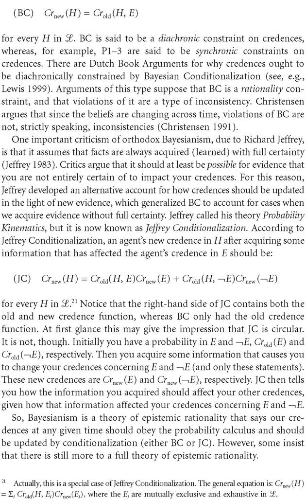
Suppose for the moment that it has been established that one's credences ought to satisfy the probability axioms. Are these the only normative con­straints on credences? One feature our beliefs have is that they change over time, especially when we learn new facts about the world. And it seems that there are rational and irrational ways of changing one's beliefs. In fact, perhaps most probabilists believe that there are rational and irrational ways to respond to evidence, beyond simply remaining in synch with the prob­ability calculus. One particularly large subgroup of these probabilists are known as Bayesians.

3.5.2 Bayesianism

Orthodox Bayesianism is the view that an agent's credences: should at all times obey the probability axioms; should change only when the agent acquires new information; and, in such cases, the agent's credences should be updated by Bayesian Conditionalization. Suppose that an agent has a prior credence function Cr_old. Then, according to this theory of updating, the agent's posterior credence function, Cr_new, after acquiring evidence E, ought to be:

3.5.3 Objective and subjective Bayesianism

Within the group of those probabilists who call themselves Bayesians is another division between so-called objective Bayesians and subjective Bayesians. As we saw in the previous sections, Bayesians believe that credences should obey the probability calculus and should be updated according to condi- tionalization, when new information is obtained. So far, though, nothing has been said about which credence function one should have before any information is obtained - apart from the fact that it should obey the prob­ability calculus.

Subjective Bayesians believe there ought to be no further constraint on initial credences. They say: given that it satisfies the probability calculus, no initial credence function is any more rational than any other. But if subjective Bayesians believe any coherent initial credence function is a rational one, then, according to them, a credence function that assigns only 1s and 0s to all statements - including statements that express contingent propositions - is also a rational credence function. Many philosophers (including those that call themselves subjective Bayesians) balk at this idea and so insist that any initial credence function must be regular. A regular credence function is any probability function that assigns 1s and 0s only to logical truths and falsehoods; all contingent sentences must be assigned strictly intermediate probability values.^[70] The idea roughly is that an initial credence function should not assume the truth of any contingency, since nothing contingent about the world is known by the agent.

However, we may worry that this is still not enough, for a credence func­tion that assigns a credence of, say, 0.9999999 to some contingent sentence (e.g., that the earth is flat) is still counted as a rational initial credence func­tion. There are two responses that Bayesians make here. The first is to point to so-called Bayesian convergence results. The idea, roughly, is that as more and more evidence comes in, such peculiarities in the initial credence function are in a sense “washed out” through the process of repeated applica­tions of conditionalization. More formally, for any initial credence function, there is an amount of possible evidence that can be conditionalized on to ensure the resulting credence function is arbitrarily close to the truth. See Earman (1992, 141-9) for a more rigorous and critical discussion of the various Bayesian convergence results.

The second response to the original worry that some Bayesians make is that there are in fact further constraints on rational initial credence func­tions. Bayesians who make this response are known as objective Bayesians. One worry with the prior that assigned 1s and 0s to contingent statements was that such a prior does not truly reflect our epistemic state - we do not know anything about any contingent proposition before we have learned anything, yet our credence function says we do. A similar worry may be had about the prior that assigns 0.9999999 to a contingent statement. This type of prior reports an overwhelming confidence in contingent statements before anything about the world is known. Surely such blind confidence cannot be rational. Reasoning along these lines, E.T. Jaynes, perhaps the most famous proponent of objective Bayesianism, claims that our initial credence function should be an accurate description of how much information we have:

[A]n ancient principle of wisdom - that one ought to acknowledge frankly the full extent of his ignorance - tells us that the distribution that maximizes H subject to constraints which represent whatever information we have, provides the most honest description of what we know. The probability is, by this process, “spread out” as widely as possible without contradicting the available information. (Jaynes 1967, 97)

The quantity H is from information theory and is known as the Shannon entropy.^[71] Roughly speaking, H measures the information content of a distribution. According to this view, in the case where we have no informa­tion at all, the distribution that provides the most honest description of our epistemic state is the uniform distribution. We see then that the prin­ciple that Jaynes advocates - which is known as the Principle of Maximum Entropy - is a generalization of the Principle of Indifference. This version of objective Bayesianism thus faces problems similar to those that plague the logical and classical interpretations. Most versions of objective Bayes- ianism ultimately rely on some version of the Principle of Indifference and so suffer a similar fate. As a result, subjective Bayesianism with the condition that a prior should be regular is perhaps the most popular type of Bayesianism amongst philosophers.

3.5.4 Other norms

At this stage, we have the following orthodox norms on partial beliefs:

1. One's credence function must always satisfy the standard probability calculus.

2. One's credence function must only change in accordance with conditionalization.

3. One's initial credence function must be regular.

However, there are still more norms that are often said to apply to beliefs. One important such norm is David Lewis' Principal Principle (LPP) (1980). Roughly, the idea behind this principle is that one's credences should be in line with any of the objective probabilities in the world, if they are known. More formally, if Ch_t(A) is the chance of A at time t (e.g., on a propensity interpretation of probability this would be the propensity at time t of A to obtain), then:

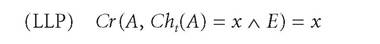
where E is any proposition, so long as it is not relevant to A.^[72] LPP, as originally formulated by Lewis, is a synchronic norm on an agent's initial credence function, though LPP is commonly used as synchronic con­straint on an agent's credence function at any point in time.

Another synchronic norm is van Fraassen's Reflection Principle (VFRP) (1995). Roughly, the idea behind this principle is that if, upon reflection, you realize that you will come to have a certain belief, then you ought to have that belief now. More formally, the Reflection Principle is:

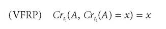
where t₂ > t₁ in time.

Another more controversial norm is Adam Elga's principle of indiffer­ence for indexical statements, used to defend a particular solution to the Sleeping Beauty Problem. The problem is that Sleeping Beauty is told by scientists on Sunday that they are going to put her to sleep and flip a fair

coin. If the coin lands “tails,” they will wake her on Monday, wipe her memory, put her back to sleep, and wake her again on Tuesday. If the coin lands “heads,” they will simply wake her on Monday. When Sleeping Beauty finds herself having just woken up, what should her credence be that the coin landed “heads”? According to Lewis, it should be 1/2 since this is the chance of the event and LPP says Sleeping Beauty's credence should be equal to the chance. According to Elga, there are three possibilities: (i) she is being woken for the first time, on Monday; (ii) she is being woken for the second time, on Tuesday; or (iii) she is being woken for the first time, on Monday. All of these situations are indistinguishable from Sleeping Beauty's point of view, and Elga argues that an agent should assign equal credence to indistinguishable situations - this is his indifference principle. So, according to Elga, Sleeping Beauty should assign equal prob­ability to each possibility, and so her credence that the coin landed “heads” ought to be 1/3. See Elga (2000) for more on the Sleeping Beauty Problem, and Weatherson (2005) for criticism of Elga's version of the Principle of Indifference.

4.