Notions and Conditions of Controllability in a Dynamic Strategic Setting

In this section we will limit ourselves to very simple notions, leaving complexities to interested readers, who can refer to Acocella, Di Bartolomeo and Hughes Hallett (2013). We sim­ply describe (1) the dynamic setting, (2) the information structures, (3) the solutions corresponding to the different structures and (4) how to calculate the minimum time needed for dynamic controllability.

4.5.1 A Simple Dynamic Setting

The simplest dynamic representation of an economy, in the form of a model, is as a linear difference equation system^[61]:

(4.7) A₀y_t = A₁y_t~₁ + B₀u_t + C₀w_t t = 1,..., T (structural form) where y_t is the vector of endogenous variables and poten­tial policy targets in the system, u_t is the vector of policy instruments available, and w_t are random shocks and other exogenous influences or variables, which also affect this economy's outcomes. The matrices A ₀, A ₁∈R^qxq, B₀∈R^qxm and C₀∈R^qxq represent parameters and may also be the identity matrix. These matrices are all nonzero, meaning that they all contain at least one, some or many nonzero elements.

It is also easy to transform system (4.7) to its ‘reduced form', equivalent to static reduced-form models:

(4.8) y_t = A₁y_t-₁ + B₀u_t + C₀w_t (reduced form) where A₁ = A₀¹A₁, B₀ = A₀¹B₀ and Co = A₀¹C₀. This reduced- form model takes account of all the contemporaneous simul­taneity in the model and always exists as long as there are no redundant equations (equations linearly dependent on other equations).

4.5.2 Notions of Controllability

If there are dynamic relationships describing how the econ­omy evolves, there are likely to be dynamic objectives that policymakers would like to reach. There are four possible types:

1. Static Objectives. Hitting desired target values at each time from any initial condition.

2. Multi-period Static Objectives. Hitting and holding desired target values across a certain time interval, if necessary by changing instrument settings.

3. Target-Point Objectives. These are fixed targets to be reached at some specific point in time in the future.

4. Target-Path Objectives. Hitting certain target values at a certain point in time and then holding a sequence of arbitrary point objectives for a certain interval thereafter.

Formally, the preceding problems can be illustrated in terms of four parameters. Assuming that the policymaker aims to reach his or her desired targets from t₀ (current period) or from t₀ on, the policymaker should act at least from the current period and anticipate his or her future policy changes. The relevant parameters can then be defined as follows: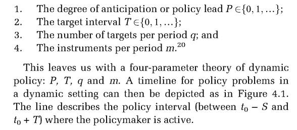

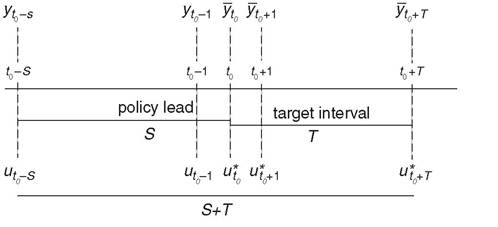
Figure 4.1 A timeline for dynamic policy problems. (Source: Acocella, Di Bartolomeo and Hughes Hallett 2013)

^[1] Normally, we assume that we have the same number of targets and instruments in each period (i.e. q and m are the same in each period). Relaxing this assumption causes additional issues to arise.

In the case of static objectives, the policymaker aims to achieve his or her target vector in the current period by setting his or her instruments in the current period. This corresponds to Tinbergen’s static fixed-objective problem since the policy­maker aims to achieve his or her target vector under linear constraints augmented by the given initial conditions.

4.5.3 Information Structures

Three information structures are relevant. These are open loop, feedback and closed loop. We can informally define them as follows:

Open-Loop Policy Rule. An open loop policy rule is one that can be calculated, optimally or not, at the first planning period and is then implemented irrespective of how the economy actually develops thereafter

Feedback Policy Rule. A feedback policy rule reacts to the latest information on past realisations of variables in the model but not to changes in expectations or probabilis­tic information on future variables or improved coeffi­cients in the model (an improved understanding of the economy's behaviour) going forward.

21

Closed-Loop Policy Rule. A closed loop policy rule takes account of all the latest information available at each t, including probabilistic information on disturbances, any revised expectations for future variables and any revisions made to the model or our understanding of the policymakers' preferences and priorities. All of this in the same feedback-rule form.

Correspondingly to these rules, we could define open­loop, feedback and closed-loop strategies. Specifically, the open-loop strategy is a sequence of decisions for each time period, each of which depends on the initial state. The open­loop Nash equilibrium is derived from the presumption that at the beginning of the game each player can make binding commitments about the actions he or she will undertake over the entire planning period. That is, each player designs his or her optimal policy based on his or her own loss function at the beginning of the period and sticks to that policy sequence throughout the entire period. Hence, open-loop strategies are not usually time consistent. Feedback strategies provide instead a strongly time consistent (i.e. sub-game perfect) equilibrium. Sub-game perfectness requires that for every possible sub-game, feedback strategies u^f will remain the equilibrium and optimal value for that sub-game. In practice, a feedback strategy means that a contingent rule (dependent on the system's state vector at time t) is provided for each player and that the rules themselves can be obtained from the backward recursions of dynamic programming (Holly and Hughes Hallett 1989). That, in turn, requires the constrained optimisation problem faced by each player at each t to be recursively additively separable with respect to each t,...,T. The recursive nature of the problem is upset if there are anticipation effects from REs or actions expected from other players in the future, when a closed-loop strategy is in order reacting to changes in expectations of future events as they appear, in addition to past outcomes.

4.5.4 Open-Loop Nash Solutions

The open-loop Nash context allows us to express each agent's optimisation problem as a static one, as he or she can set his or her optimal rule u‘* at the beginning of the game, taking as given the rules used by the other agents ιU^j for j2n∣i.

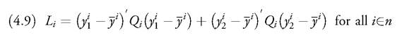
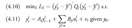
If, for simplicity, the dimensions of the target and the instrument vectors and the vector of the desired targets are time invariant,and we ignore stochastic disturbance and expectations (in a way certainty equivalence can always be advocated), each agent must minimise, given the initial condition y₀

under the constraint

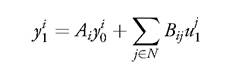
in the first period and

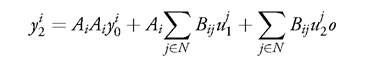
in the second period.

Let us see this with reference to cases where there are excess or fewer instruments with respect to targets in each period. Imagine, for example, that the policymaker has two targets over a two-period model (four targets); in the first period he or she has three instruments, and in the second one he or she can statically control the system only in period 1, but multi-period controllability is assured, as any four- target vector can be achieved in the two periods. This is because the effects of instruments are no longer purely static, and thus, both static and dynamic multipliers must be taken into account.

Ensuring that the number of instruments is at least equal to that of targets in each period is stronger than the conditions required for ensuring multi-period static controllability. This could be obtained also when the golden rule is satisfied neither in each period nor in aggregate, just as an effect of the dynamic nature of the instruments. However, if static con­trollability is satisfied, multi-period static controllability is also ensured.

We now refer to Figure 4.1 and derive the minimum time needed to reach targets by using the concept of dynamic controllability. In a classical, non-parametric context, dynamic controllability is obtained for any t equal to or larger than S and can be derived by solving the following optimisa­tion problem:

A trivial case arises if m = q, as then S = 1 solves this problem. Thus, the policymaker always satisfies dynamic controllabil­ity. By contrast, if m < q, the policymaker should exploit the dynamic multipliers to obtain the desired targets, and this requires S > 1.

instruments the policymaker has. For instance, if only one instrument is available, he or she can expect to reach one target value in period one, two after two periods and so on; i.e. dynamic controllability requires at least S = q periods. In general, if the policymaker has m instruments, dynamic controllability requires at least S = q/m periods. For a formal proof of this, see Preston and Pagan (1982).

By applying the preceding result to a multi-player context, it emerges that if two (or more) players aim to solve a problem of the kind (4.10), where q(1)/m(1) = S and q(2)/m(2) = S, both would be able to achieve their targets, and no equilibrium would exist. By contrast, if q(i)/m(i) ≤ S for all i, the existence of an equilibrium for problem (4.10) with multiple players is ensured. In other cases, the conditions for equilibrium exis­tence will be more complex. But we do not analyse them here.

The second case of interest is where player i aims to reach certain target values in the shortest possible time. Assuming dynamic controllability, what can be achieved now depends on how many target values player i attempts to reach. Again, if a player has only one instrument available, he or she can expect to reach one target value in period one, two after two periods and all targets after a number of periods equal to the integer value of q(i)/m(i) targets if q(ιj > m(i). In the absence of static controllability, this is as far as he or she can go in minimising the time taken to reach various targets.

If dynamic controllability applies in period S, player i can achieve his or her target values y_i exactly, in expectation, in period S at least. This means, applying certainty equiva­lence, that player i can achieve a value of E(L_s) = 0 in his or her loss function and maximum expected utility in period t = S. But the same result does not hold if there are instrument costs, since both static and dynamic controllability no longer apply. Nor does this result say anything about the costs along the way. In general, we should expect E(L_t) ≠ 0, for all t = 1,..., S - 1 and m(i)S ≤ Tq(i). Analysingthe utility costs in either of those two cases requires a full specification of the preferences in the loss functions E(L_t) for each t.

There is one exception to the assertion that when the system is only dynamically controllable the policymaker must wait to achieve his or her target values. Section 4.5.6 shows that in an economy with forward-looking REs of future outcomes, dynamic controllability may be available from period one if announcements of future policy actions are used alongside the actual (current and past) policy interven­tions. If this is the case, and in the absence of instrument costs, then the costs along the way will fall away: E(L_t) = 0, for all t= 1,...,T.

4.5.4 Feedback Nash Equilibrium

In a dynamic setting, controllability (or the golden rule of economic policy), policy ineffectiveness and the existence of a feedback Nash equilibrium are related to one another through the following two theorems.

Theorem 4.5 (ineffectiveness in feedback Nash equili­brium). In a LQ-difference game where an equilibrium exists, if one player satisfies the golden rule, then all other players' policies are ineffective for all the target variables shared with that player.

Theorem 4.6 (nonexistence in feedback Nash equili­brium). The feedback Nash equilibrium of the policy game described earlier does not exist if two or more players satisfy the golden rule and aim to achieve different target values for at least one shared target variable.

Proofs: See Acocella, Di Bartolomeo and Hughes Hallett (2013).

Theorem 4.6 highlights the importance of these results for economic policy. This theorem says that if two independent policy authorities - say, fiscal policymakers and the central bank - decide to pursue different inflation targets, then the Nash equilibrium does not exist if both control the economy. When this is the case, the economy will not be able to reach a stable equilibrium position even when both policymakers try to optimise their policies. Moreover, the conditions for this are not particularly stringent. In fact, target indepen­dence may actually be unhelpful - not because fiscal and monetary policies cannot be coordinated properly but because the underlying equilibrium cannot be reached if both policymakers try to optimise their policy choices simul­taneously and independently.

4.5.5 Dynamic ControIIabiIitywith Closed-Loop Information

Policymakers routinely use announcements^[63] as policy instruments to influence future expectations and, through them, future results. Announcement and signalling effects in fact imply that the announcement of a change in policy will typically affect agents' behaviour, even before the change is actually made. Rational policymakers should therefore internalise announcement effects and use the sig­nals strategically. The economic policy literature, however, does not have a formal model of whether, and under what conditions, policy announcements can be used to system­atically affect economic performance.

Time inconsistency and REs are said to imply that such commitments cannot be considered credible and would inevitably lead to Pareto-inferior outcomes. We discuss the credibility problem by considering REs within the tradi­tional Tinbergen framework and show that under certain circumstances REs will not only present the policymakers with no problem of how to set their policies consistently but may actually add to the scope of their policy instruments, in effect, giving them additional sources of effective policy power.

Let us consider an economy represented by a generic linear RE model in reduced form:

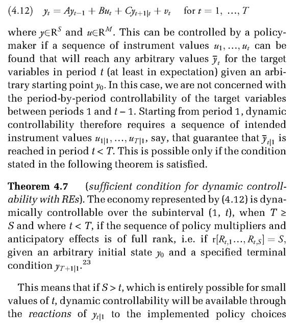
²³ This theorem provides a sufficient condition for dynamic controllability. The corresponding necessary condition involves a smaller subset of R_tj having full rank depending on how many policy instruments are available.

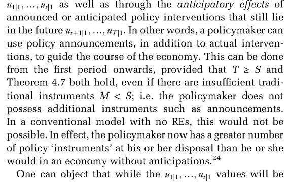
implemented decisions, the remaining u_t+1∣₁,..., m_t∣₁ values are only announcements that may never actually be carried out. However, because they lie in the future from the per­spective of y_t∣₁, any subsequent time inconsistency plays no role in the controllability of y_t∣₁ as long as they are genuinely held expectations at that point and the policymaker will be able to reach his or her desired values for y_t in expectation.

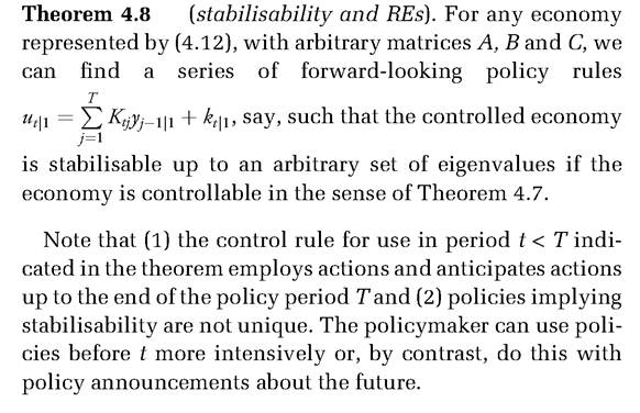
4.5.7 Stabilisability under REs

The reasoning underlying Theorem 4.7 can be applied to show that any economy can also be stabilised to an arbitrary degree under rational, forward-looking expectations if it is dynamically controllable in the sense of this theorem. An arbitrary degree of stabilisation means that policy rules can be found to make the economy follow an arbitrarily stable path based on an arbitrary set of eigenvalues such that it returns to the original path following a shock. Theorem 4.8 gives the RE analogue of the standard stabilisability theorem for backward-looking or physical systems.

24

Forward guidance is an announcement ofthis type (see Chapters 5 and 6).