SIMULATION OF JOINT LOSSES FOR THE BANKING SYSTEM

Distributions of losses are a very important tool in risk management because such distributions allow the risk managers to compute several stan­dard and well understood risk measures.

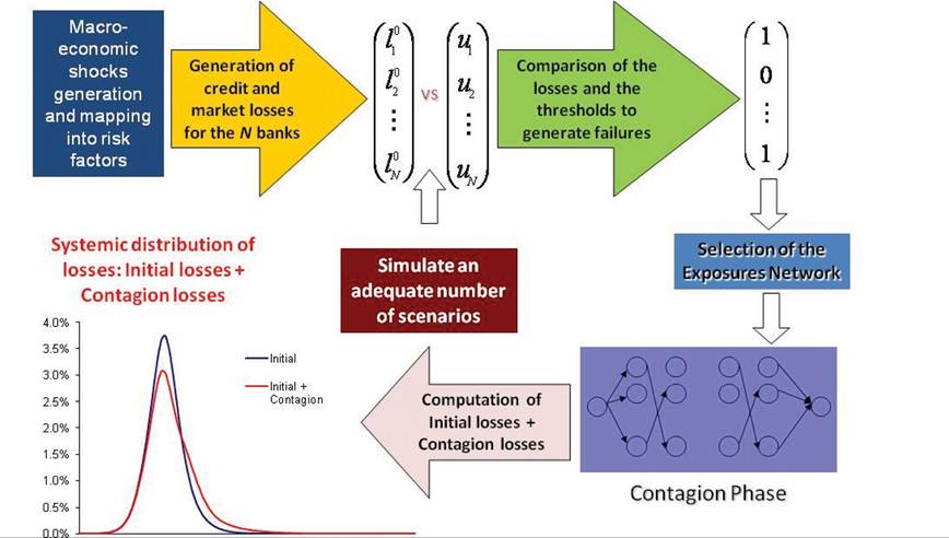
In order for us to estimate the distribution of losses for the system, we need to be able to gen­erate joint losses. Joint losses are correlated by common or similar exposures and especially in times of financial hardship. We have developed a simulation model to allow the estimation of the distribution of losses of the system as a whole.

In previous works (Marquez-Diez-Canedo & Martinez-Jaramillo, 2007; Marquez-Diez- Canedo, et al., 2009), we have estimated the distribution of losses for the banking system first using just the probabilities and secondly by using the individual distribution of losses for each bank.

While this approach has several advantages such as relying on detailed historical information and using this information to generate adverse shocks to the financial system, it lacks a clear link between these shocks and real economic variables. It is not possible to know what kind of underlying events are causing the shocks being evaluated. It also faces technical and data chal­lenges: to compute the joint distribution, a copula to merge market and credit losses distributions is used. A very important part of the process is the calibration of the copula with banks’ financial data, such as ROA, in order to capture the joint dependence structure. This information is not fully available for all the banks in the system, mainly because new banks⁷ have not been reporting these indicators for long enough, hence previous studies were limited to a subset of the banks in the system.

Figure 1. The simulation algorithm

Having a model linked to economic variables overcomes some of these difficulties.

Once losses caused by the initial shock are determined, the contagion process takes place through the interbank market, and the final effect on the financial system as a whole depends on the magnitude of the effects caused by the initial losses combined with the interbank exposures and the interconnectedness of these exposed banks.

The interbank lending market plays a crucial role in liquidity transmission between banks. This market is the most recognized (or at least one of the most studied) channel for financial contagion. Moreover, there is a worldwide concern on char­acterizing the financial network of exposures in order to derive measures of financial fragility. However, such network changes constantly and some examples will be provided.

2.1. Data

The data used to obtain the system’s distribution of losses for the Mexican banking system consists on the daily interbank exposures, the macroeconomic information used to build the macro model (GDP, interest rates, stock indexes, etc.) affecting credit and market risk factors, which have an effect on banks portfolio and Tier 1 capital.

Regarding the interbank market, the Mexican central bank has daily data that can be used to calculate the matrix of interbank exposures of the Mexican financial system, from January 2005 onwards⁷. The interbank exposures considered in this study comprise all the uncollaterized inter­bank lending, securities being hold, which are issued by other banks, the credit component of derivative transactions and credit lines as part of the interbank market.

For example, a common approach along this line of research is making the assumption of maxi­mum entropy on the distribution of the interbank exposures but this is not a realistic one (as it is pointed out in Graf, et al., 2005⁸, contagion in a network built under the maximum entropy prin­ciple and without such assumption), at least not in the Mexican case.

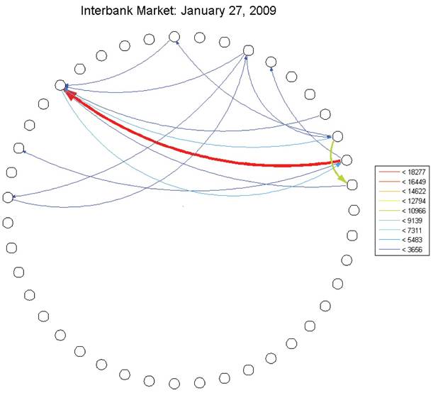
Figure 2 shows a typical network of expo­sures and in Figure 3 we can see only the largest exposures for such day. This is the network rep­resenting the interbank market that will be used during this work.

The exposures on the Mexican interbank expo­sures network vary widely as the Mexic an banking system is quite heterogeneous. As one might ex­pect, big banks tend to have larger exposures than medium or small size banks. It is also important to note that the size of the exposure by itself is not as important as the size of the exposure relative to the Tier 1 capital of a bank. Exposures, which represent an important proportion of the Tier 1

Figure 2. The Mexican interbank market (quantities are in millions of pesos)

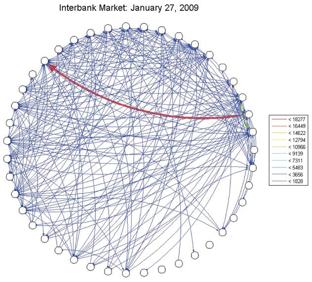
Figure 3. Large exposures at the Mexican interbank market (quantities are in millions of pesos)

capital, are the exposures, which could detonate contagion in the case of failure of the institution that is borrowing from a particular bank.

Concentration plays also an important part in contagion as it is possible that a bank which has many counterparts is lending or borrowing in a concentrated fashion and as a consequence is more vulnerable to experience important losses as a consequence of the failure of one of its borrowers. Moreover, it could also be problematic for a bank to have its funding sources very concentrated as the failure of an important lender could compromise the liquidity needs of a bank.

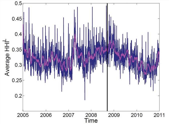
The Herfindahl-Hirschman Index (HHI) is a measure which is normally used in the context of competition in a market or industry but in this context we will use it as a measure of concentra­tion. A HHI close to one is associated with a full concentration in lending or borrowing, whereas a HHI close to zero indicates a diversification among the counterparts of a bank. Figure 4 shows the evolution of the average HHI for the banking system. Although, a relative low concentration is shown in this figure, things are different from bank to bank. The range of possibilities goes from banks, which tend to diversify in lending or borrowing, to banks which lend or borrow in a highly concentrated fashion. Even a bank can behave differently on lending and borrowing hav­ing a HHI for lending close to one and a HHI for borrowing close to zero.

In addition to the HHI, one important measure, which can be useful to describe concentration and preference for lending and borrowing, is the Prefer­ence Index proposed in Cocco et al. (2009). This measure provides an estimate of the intensity of the relationship between two banks over a period of time and this is important in particular during periods of stress. This index can be computed from the lending or the borrowing side for each pair of banks, a PI close to one is associated with a high preference for a particular counterpart, whereas an index close to zero is associated with a low preference for a specific counterpart.

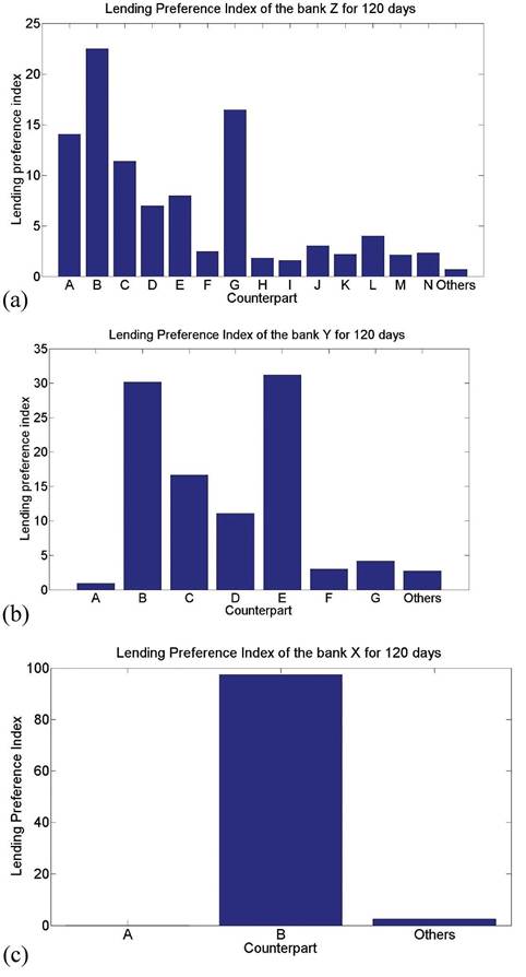
The time window plays an important role on the preference index, the authors in Cocco et al. (2009) originally proposed a window of 30 days, in the examples shown here, a window of 120 days is used. Figure 5 shows the lending prefer­ence indexes for three different banks: X, Y, and Z. From this figure, it is shown that bank Z has its lending relatively diversified, but it has a strong relationship with bank B as of all the exposures

Figure 4. Evolution of the average HHIfor the banking system

this bank had in 120 days period, more than 20% were only with bank B.

Figure 5. Preference indexfor various banks: (a) Lending PIfor a 120 daysperiodfor bank Z; (b) Lend­ing PI for a 120 days period for bank Y; (c) Lending PI for a 120 days period for bank X

These two simple measures provide us with a clear idea of the heterogeneity in concentration for the system. It was shown that, despite the system’s HHI being relatively low, concentration changes from bank to bank and even within the same bank from lending to borrowing.

2.2. The Link to Economic Variables

When the goal of the analysis goes beyond the day-to-day activity and is more policy oriented, it becomes more appealing having a shocks genera­tion process that has a direct interpretation within the context of the real economy that complies with minimal consistency requirements and that has the flexibility to explore different sets of conditions.

Depending on the scope of the work and the type of analysis to perform, there are several alternatives to establish the link between losses and the real economy. Some approaches are more theoretically sound or more robust than others, and options range from highly sophisticated dynamic GE models to relatively simple statistical models. Ultimately, considerations such as information availability, and the trade-off between tractability and predictive power, led us to opt to model the links between losses and economic variables using structural Vector Autoregressive (VAR) models.

Despite its limitations, we considered it was the most suited approach given the characteris­tics of the problem we were analyzing. We are modeling the short-term effects of shocks in the credit and market portfolios of banks in order to evaluate the possible contagion effects that these shocks can have.

It also offers relatively simple yet powerful alternatives to evaluate extreme conditions⁹. It is highly likely that “brute force” simulation leads to no occurrence of shocks with a systemic impact; but it is still of interest knowing the possible ef­fect of some events on the tails of the distribution. The parametric assumptions and the structure of the model allow evaluating these events while as­signing weights to their probability of occurrence. For example, if one is willing to explore what would happen if variable x increases in at least 4 standard deviations, a whole simulation process can be done conditional on x, and its probability can be determined.

Finally, the point to emphasize here is that, for policy analysis, it is necessary to have a link between the distribution of losses and the real economy, but the way to do it is far from unique. In general, the more data intensive the evaluation process of systemic risk, the more beneficial a relatively simpler model is.

2.2.1. Scenarios Generation

As described in Appendix A, scenarios are gener­ated following the same spirit of impulse-response function construction methodology. Two sets of scenarios were generated (below there is a lengthier discussion about this): 30,000 “standard” scenarios, according to the underlying normal distribution (See Figures 6 and 7); plus 5,000 “tail” scenarios, where the different variables were set to receive severe shocks (for example, a simultaneous four standard deviations increase or decrease), and the rest of the random shocks were generated conditional on these realizations¹⁰.

3.