Predicting the outcome of competition
The outcome of competition can be predicted if we know how the population sizes of species 1 and species 2 are likely to change over time. For example, if the population size of species 2 is likely to increase while that of species 1 is likely to decrease to zero, then species 2 should drive its competitor to extinction, thus “winning” the competitive interaction.
A computer can be programmed to solve Equation 14.1, thereby predicting the population sizes of species 1 and 2 at different times. Here, however, we'll use a graphical approach to examine the conditions under which each species would be expected to increase or decrease in population size.We begin by determining when the population size of each competing species would stop changing in size. This approach, which we also used for the Lotka- Volterra predator-prey model (see Concept 12.3), is based on the idea that the population size (N) does not change when the population growth rate (dN∕dt) equals zero (or reaches an equilibrium). For example, based on the Lotka- Volterra competition model (Equation 14.1), the population size of species 1 does not change when dN1∕dt = 0. When we set dN1∕dt equal to zero, we find that the population size of species 1 (N1) does not change when

(14.2)
Likewise, the population size of species 2 (N2) does not change when
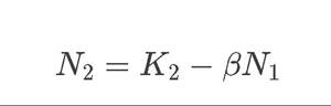
(14.3)
Notice that Equations 14.2 and 14.3 are straight lines, written with N1 as a function of N2 and N2 as a function of N1, respectively. Each of these lines is called the zero population growth isocline (or simply isocline), so named because a population does not increase or decrease in size for any combination of N1 and N2 that lies on these lines.
For species 1, the abundance does not change when dN1∕dt = 0, which occurs when N2 = K1/α and N1 = K1 Similarly,for species 2, the abundance does not change when dN2∕dt = 0, which occurs when N1 = K2∕β and N2 = K2.
Once we determine K1∕α and K2∕β, we can then plot the isoclines for both species 1 (x-axis) and species 2 (ó-axis) in graphical form. For species 1, the isocline will be a diagonal line originating at the value N2 = K1∕α and ending at the value N1 = K1 (FIGURE 14.13A). This isocline represents the number of individuals of species 2 that would keep species 1's population from changing (or at equilibrium). For example, in Figure 14.13A, because a point to the right of the N1 isocline represents more individuals than zero population growth will allow, the population size of species 1 will decrease until it reaches the isocline. This is true for the entire region shaded in blue: the population size of species 1 decreases for all points to the right of the N1 isocline. In contrast, when the population size of species 1 is to the left of the N1 isocline, the population size of species 1 increases. Similar reasoning applies to species 2's isocline, which can be plotted as the diagonal line originating at the value N1 = K2∕β and ending at the value N2 = K2 (FIGURE 14.13B). This isocline represents the number of individuals of species 1 that would keep species 2's population from changing (or at equilibrium). Here the population size of species 2 decreases in regions above the N2 isocline and increases in regions below the N2 isocline.
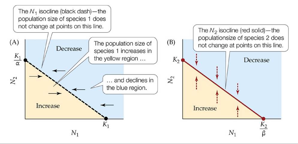
FIGURE 14.13 GraphicalAnalysesofCompetition Thezeropopulationgrowthisoclines from the Lotka-Volterra competition model can be used to predict changes in the population sizes of competing species.
(A) The Ni isocline. The change in population size of species 1 (indicated by black solid arrows) increases in the yellow region and decreases in the blue region. (B) The isocline. The change in population size of species 2 (indicated by red dashed arrows) increases in the yellow region and decreases in the blue region. View larger imageThe graphical approach we have just described can be used to predict the end result of competition between species. To do this, we plot the N1 and N2 isoclines together. Because there are four possible ways that the N1 and N2 isoclines can be arranged relative to each other, we must make four different graphs. In two of these graphs, the isoclines do not cross, and competitive exclusion results: depending on which isocline is above the other, either species 1 (FIGURE 14.14A) or species 2 (FIGURE 14.14B) always drives the other to extinction. Note that in the regions shaded in blue, the population sizes of both species are greater than the population sizes on their isoclines, and hence both species decrease in number (as indicated by the thick black arrows). Similarly, in the regions shaded in yellow, the population sizes of both species are less than those on their isoclines, and hence both species increase in number. In the regions shaded in light or dark gray, one species increases in number (because its
population sizes are less than those on its isocline) while the other decreases until the species that increases reaches its carrying capacity (K) and the species that decreases reaches zero and becomes extinct.
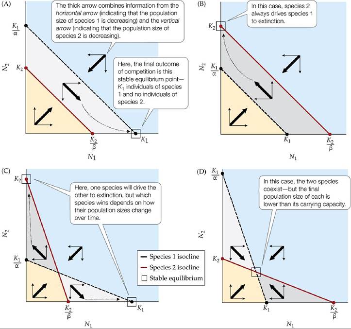
FIGURE 14.14 Outcome of Competition in the Lotka-Volterra Competition Model The outcome of competition depends on how the N1 and isoclines are positioned relative to one
another. (A) Competitive exclusion of species 2 by species 1; species 1 always wins.
(B) Competitive exclusion of species 1 by species 2; species 2 always wins. (C) The two species cannot coexist; either species 1 or species 2 wins depending on population sizes of both species. (D) Species 1 and species 2 coexist. The box in each graph indicates a stable equilibrium point— a combination of population sizes of the two species that, once reached, does not change over time.In (B), if K2 = 1,000 and if species 1 went extinct when N2 = 1,200, how would the population size of species 2 change after the extinction of species 1?
View larger image
Competitive exclusion also occurs in the third graph (FIGURE 14.14C), but which species “wins” depends on whether the changing population sizes of the two species first enter the region shown in dark gray (in which case, species 2 drives species 1 to extinction) or the region shown in light gray (in which case, species 1 drives species 2 to extinction). Finally, FIGURE 14.14D shows the only case in which the two species coexist, and hence competitive exclusion does not occur. Although in this case neither species drives the other to extinction, competition still has an effect: the final or equilibrium population size of each species (indicated by the box in the figure) is lower than its carrying capacity, as in Gause's experiments with Paramecium (see Figure 14.9A).
Researchers have used the graphical approach described in Figure 14.14 to predict the outcome of competition under different ecological conditions. For example, Livdahl and Willey (1991) used this approach to predict whether competition with a native species of mosquito could prevent the invasion of an introduced mosquito species. You can explore their results in ANALYZING DATA 14.1.
Ą ∖
ANALYZING DATA 14.1
Will Competition with a Native Mosquito Species Prevent the Spread of an Introduced Mosquito?
The mosquito Aedes albopictus breeds in small volumes of water, such as those in tree holes (cavities in trees that can hold water) and in abandoned tires.
Introduced from Asia to North America in the 1980s, this species is a public health concern because it can transmit diseases such as dengue fever. Once in North America, A. albopictus colonized tree holes and tires, where it encountered thriving populations of several different native species of mosquitoes.Livdahl and Willey (1991)* sought to predict the outcome of competition between A. albopictus and the native mosquito A. triseriatus, a predominant member of tree hole communities. To do this, they estimated competition coefficients and carrying capacities for A. albopictus and A. triseriatus mosquito larvae developing in water obtained from tree holes and from tires. Their results are shown in the table.
| Water obtained from tree holes | Water obtained from tires |
| Competition coefficients | |
| α = 0.43 | α = 0.84 |
| β = 0.72 | β = 0.25 |
| Carrying capacities (no. individuals/100 ml water) | |
| K1 = 42.5 | K1 = 33.4 |
| K2 = 53.2 | K2 = 44.7 |
1. Using Equation 14.1, designate A. triseriatus as species 1 and A. albopictus as species 2. Use the data in the table to plot the N1 and N2 isoclines (see Equations 14.2 and 14.3) for these two species competing in tree hole communities. Predict the equilibrium population density (no. individuals per 100 ml of water) for each species. Describe the likely outcome of competition between these two species in tree hole communities.
2. On a separate graph, plot the N1 and N2 isoclines for these two species competing in tires. Predict the equilibrium population density (no. individuals per 100 ml of water) for each species. Describe the likely outcome of competition between these two species in tires.
3. Is it likely that competition with the native species (A. triseriatus) will prevent the spread of the introduced species (A. albopictus)? Explain.
*Livdahl, T. P., and M. S. Willey. 1991. Prospects for an invasion: Competition between Aedes albopictus and native Aedes triseriatus. Science 253: 189-191.