A MODEL AND ALGORITHM FOR EQUAL-OPPORTUNITY POLICY
Consider a population whose members are partitioned into a finite set of types. A type comprises the set ofindividuals with the same circumstances, where circumstances are those aspects of one’s environment (including, perhaps, one’s biological characteristics) which are beyond one’s control, and influence outcomes of interest.
Denote the types t = 1,.... T. Let the population fraction of type t in the population be ft. There is an objective for which a planner wishes to equalize opportunities. The degree to which an individual will achieve the objective is a function of her circumstances, her effort, and the social policy: We write the value of the objective as ut(e, φ), where e is a measure of effort and φ 2 Φ the set of social policies. Indeed, ut(e, φ) should be considered to be the average achievement of the objective among those of type t expending effort e when the policy is φ. Here, we will take effort to be a nonnegative real number. Later, we will introduce luck into the problem.u is not, in general, a subjective utility function: Indeed u is assumed to be monotone increasing in effort, whereas subjective utility is commonly assumed to be decreasing in standard conceptions of effort. Thus, u might be the adult wage, circumstances could include several aspects of childhood and family environment, and e could be years of schooling. Effort is assumed to be a choice variable for the individual, although that choice may be severely constrained by circumstances, a point to which we will attend below. The final data for the problem consist of the distributions of effort within types as a function of policy: For the policy φ, denote the distribution function of effort in type t as Gφ(∙). We would normally say that effort is chosen by the individual by maximizing a preference order, but preferences are not the fundamentals of this theory: Rather, the data are {T, Gtφ,ft, u, Φ}, where we use T to denote, also, the set of types.
Defining the set of types and the conception of effort assumes that the society in question has a conception of the partition between responsible actions and circumstances, with respect to which it wishes to compute a consonant approach to equalizing opportunities. We describe the approach of Roemer (1993, 1998). The verbal statement ofthe goal is to find that policy which nullifies, to the greatest extent possible, the effect of circumstances on outcomes, but allows outcomes to be sensitive to effort. Effort comprises those choices that are thought to be the person’s responsibility. But note that the distribution of effort in a type at a policy, Gtφ, is not due to the actions of any person (assume here a continuum of agents), but is a characteristic of the type. If we are to indemnify individuals against their circumstances, we must not hold them responsible for being members of a type with a poor distribution of effort.
We require a measure of accountable effort, which, because effort is influenced by circumstances, cannot be the raw effort e. (Think of years of education—raw effort—which is surely influenced in a major way by social circumstances.) Roemerproposedto measure accountable effort as the rank of an individual on the effort distribution of her type: thus, if for an individual expending effort e, Gtφ(e) = π, we say the individual expended the degree of effort π, as opposed to the level of effort e. Therankprovides away of making inter-type comparisons ofthe efforts expended by individuals. Aperson is judged accountable, that is to say, by comparing her behavior only to others with her circumstances. In comparing the degrees of effort of individuals across types, we use the rank measure, which sterilizes the distribution of raw effort of the influence of circumstances upon it.[136]
Because the functions u are assumed to be strictly monotone increasing in e, it follows that an individual will have the same rank on the distribution of the objective, within his type, as he does within the distribution of effort of his type.11 Define:
which is also the inverse of a distribution function.) Inequality of opportunity holds when CheseJunctions are not identical.
In particular, because we are viewing persons at a given rank π as being equally accountable with respect to the choice of effort, the vertical difference between the functions is a measure of the extent of inequality of opportunity
 (or, equivalently, the horizontal distance between the cumulative distribution functions).
What policy is the optimal one, given this conception? We do not simply want to render the functions v identical at a low level, so we need to adopt some conception of “maxi-minning” these functions. We want to choose that policy which pushes up the lowest vt function as much as possible—and as in Rawlsian maximin, the “lowest” function may itself be a function of what the policy is. A natural approach is therefore to maximize the area below the lowest function vt, or more precisely, to find that policy which maximizes the area under the lower envelope of the functions {vt}. The formal state- rnμnf ę t(^∖'
(Computing (4.1) is equivalent to maximizing the area to the left of the left-hand envelope of the type distributions of the objective, and bounded above by the horizontal line of height one.)
Thus, the approach implements the view that differences between individuals caused by their circumstances are ethically unacceptable, but differences due to differential effort are all right. Full EOp is achieved not when the value of the objective is equal for all, but when members of each type face the same chances, as measured by the distribution functions of the objective that they face.
11
If actual effort is a vector, then a unidimensional measure e would be constructed, for example, by regressing the objective values against the dimensions, thus computing weights on the dimensions of raw effort.
One virtue of the approach taken here is that it is easy to illustrate graphically.
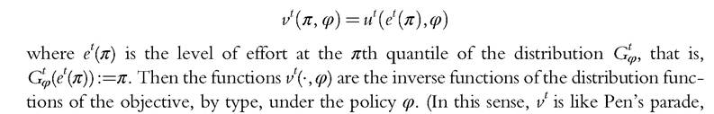
In Figure 4.1, we present two graphs, to illustrate inequality of opportunity in Hungary and Denmark. In each graph, there are three cumulative income distributions, corresponding to male workers of three types: those whose more educated parent had no more than lower secondary education, those whose more educated parent just completed
Figure 4.1 (a) Three income distribution functions for Danish male workers, according the circumstance of parental education. (The curve with darkest hue is the income distribution of sons of the least-educated parents; the lightest hue is the income distribution of sons of the most- educated parents.) (b) As in (a), but for Hungary.
secondary education, and those whose more educated parent had at least some tertiary education. (The data are from EU-SILC-2005.) The inverses of these distribution functions are the functions vt(∙, φ) defined above. The policy is the status-quo policy. It seems clear that, with respect to this one circumstance (parental education), opportunities for income have been more effectively equalized in Denmark than in Hungary.[137] The graphs are taken from Roemer (2013).
The approach inherent in (4.1) is one that treats all causes ofinequality not accounted for by a person’s type as being due to effort. For example, with respect to Figure 4.1, there are many circumstances that influence outcomes not accounted for in the definition of type, and so the inequality of opportunity illustrated in that figure should be considered to be a lower bound on the true inequality of opportunity. Nevertheless, it is often the case that delineating only a few circumstances will suffice to illustrate obvious inequality of opportunity, and one can say that social policy should attempt to mitigate at least that inequality.
Let us note that the equal-opportunity approach is non-welfarist or more precisely non- Consequentialist.
A welfarist procedure for ordering social policies uses information only in the objective possibilities sets of the population associated with those procedures. In the income example, it would use only the data of the income distribution of the population and ignore the data of what individuals were of what types. Circumstances are nonwelfare (or nonobjective) information. More informally, consequentialism only considers the final results of policies (incomes), and not the causes of those consequences. Here, we say there are two kinds of cause of outcomes with different moral status: circumstances and effort. We must distinguish between these causes and social policy should attempt to mitigate the inequality effects of one of them, but not necessarily of the other.At this point, we return briefly to consider a philosophical critique of this approach— and indeed of the general evolution of responsibility-sensitive egalitarianism, as it was reviewed in Section 4.1 above—offered by Hurley (2002), who writes that “Roemer’s account does not show how the aim to neutralize luck could provide a basis for egalitarianism.” Hurley says that, absent luck, many possible distributions of the objective could have occurred, and one cannot claim that “neutralizing” luck means to render outcomes sensitive only to degrees of effort. Moreover, she writes that it is not an argument for EOp that it neutralizes the effects of luck.
The moral premise of the EOp view is that rewards should be sensitive only to the autonomous efforts of individuals. This is a special case of rewards according to deserts. People deserve, in the EOp view, to acquire the objective in proportion to how hard they try. Thus, strictly speaking, the EOp view is not one whose fundamental primitive is equality: deservingness is fundamental, together with the normative thesis that justified inequality tracks deservingness. Inequalities that are not due to unequal efforts are defined as being due to luck; that is, luck is so-called because it is a cause of reward that is illegitimate from the EOp view.
The statement that “EOp intends to neutralize the effects of luck on outcomes” is therefore equivalent to the statement “EOp intends to render outcomes sensitive only to effort.”12
So, for example, suppose a child, A, does well in life because his parents were rich, not because he exerted great effort, while another child, B, from a poor family, does well by virtue of exerting great effort. Some might argue that it may be no less a matter of luck that B was the kind of person who works hard than that A had rich parents, but that approach, whatever its merits, is not the sense in which responsibility-concerned egalitarians use the word “luck.” Luck, for us, means the source of noneffort-caused advantage. Tobe sure, it is not an argument for EOp that it neutralizes luck; it is rather definitional of the EOp view that it does so. The argument for EOp must be that it is right to render outcomes sensitive only to effort.[138]
The next example, which is hypothetical, is given to illustrate the difference between the equal-opportunity approach and the approach that is conventional in many areas of social policy, utilitarianism. A utilitarian policy maximizes the average value of the objective in a population. Utilitarianism is a special case of welfarism, although there are many welfarist preference orderings of policies.
We consider a population partitioned into T types, where the frequency of type t is ft. The population suffers from I diseases, with the generic disease denoted i. The types might be defined by socioeconomic characteristics,[139] and the Health Ministry is interested in mitigating the effect of socioeconomic characteristics on health. There is available in the health sector an amount of resource (money), R per capita. We do not address how much of a society’s product should be dedicated to health, but only how to spend the amount that has been so dedicated. Effort is here conceived of as lifestyle quality (exercise, smoking behavior, etc.). We choose the policy space to be allocations of the resource to treating various diseases; that is vectors R = (R1,..., Ri), which will be constrained by a budget condition, where Ri is the amount that will be spent to treat each case of disease i, regardless of the characteristics of the person who has contracted the disease. Thus, by definition, we restrict ourselves to policies that are horizontally equitable: Any person suffering from disease i, regardless of her type and lifestyle quality, will receive the same treatment, because treatment expenditure is not a function of these variables. A more highly articulated policy space could allocate medical resources predicated also on the type of the patient and the lifestyle that patient had led. But in the health sector, doing so would set the stage for antagonistic patient-provider relations, and interfere with other values we hold, and so we choose to respect horizontal equity. We will return to this point below.
For any given vector, R = (R1,..., Ri) there will ensue a distribution of lifestyle quality in each type t, and a consequent distribution of disease occurrences in each type. Lifestyle quality may not be responsive to the policy, but we allow for the general case in which it is. Let us denote the fraction of individuals in type t who contract disease i when the policy is R by plt(R). Then the policy is feasible when:
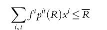
and it exhausts the budget precisely when:
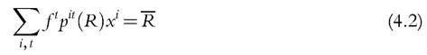
The set of admissible policies comprises all those for which (4.2) holds: This is the set Φ.
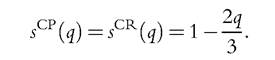
We next suppose that we know the health production functions for each type; these are functions that give the probability that a person of type t will contract disease i if she lives a lifestyle of quality q. Let i = 0 represent the case of “no disease” being contracted. We denote these functions s't(∙); thus s't(q) is the probability that a t-type will contract disease i if she lives lifestyle quality q. We presume it is the case that {s't} are monotone decreasing functions for i > 0; that is, raising lifestyle quality reduces the probability of disease.
We also have as data of the problem the mapping from the policy space Φ to the space of cumulative distribution functions on the nonnegative real numbers. Denote that class of distribution functions by Γ. The map
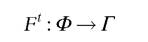
gives us the distribution of lifestyle qualities that will occur in type t, at any policy R in Φ. We write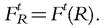 Thus, an individual with lifestyle quality q in type t lies at rank π of
the effort distribution of her type, when the policy is We denote this value
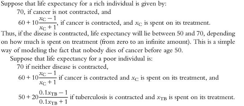
Finally, we need to postulate the relationship between treatment of disease and health outcome. Let us take the outcome to be life expectancy. We therefore suppose that we know the life expectancy for those in type t who have contracted disease i and who are treated with the resource expenditure specified by R. Denote this life expectancy by  (Denote by λ0t the life expectancy of a person of type t who contracts no disease.) We could further complexify, here, by assuming that life expectancy is a function, in addition, of the lifestyle quality of the individual, but choose not to do so.
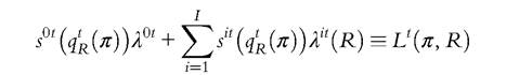
Consider, now, a policy R = (x1,..., x1), which induces a distribution of lifestyle quality in each type. Consider a type t and all those at rank π of t’s lifestyle quality distribution. Assume there is a large number of people in each type, so that the fraction of people in a type who contract a disease is equal to the probability that people in that type will contract the disease. Then,[140] the average life expectancy of all such people—the (t,π) cohort—will be
We can now define the EOp policy, which is:
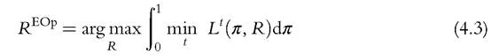
Although we need a lot of data to compute the EOp policy, it is only the Ministry of Health who must have these data: once the policy is computed, a hospital need only diagnose a patient to know what treatment is appropriate (i.e., how much to spend on the case). No patient need ever be asked her type or her lifestyle characteristics. There is, that is to say, no incursion of privacy necessitated by applying the policy—apart from the initial incursion in the research survey on a population sample that assembles the data set to compute the health production functions. The policy is horizontally equitable. This is an important point, because some philosophers have falsely concluded that applying the equal-opportunity approach will necessitate incursions into privacy, and making distinctions among individuals in resource-allocation questions that are either difficult or socially objectionable in some way (see Anderson, 1999). But this is incorrect: The planner can choose the policy space in a way that makes such distinctions irrelevant for implementing the policy. In other words, not only is the delineation of circumstances a political/social decision that may vary across societies, but so must the specification of the policy space take into consideration social views concerning privacy and fairness.
Let us make this example numerical. We posit a society with two types, the rich and the poor. The poor have lifestyles whose qualities q are uniformly distributed on the interval [0,1], while the rich have lifestyle qualities that are uniformly distributed on the interval [0.5, 1.5]. The probability of contracting cancer, as a function of lifestyle quality (q) is the same for both types, and given by:
Only the poor are at a risk of tuberculosis; their probability of contracting TB is: 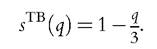
Thus, the poor can die at age 30 if they contract TB and it is not treated. With large expenditures, a person who contracts TB can live to age 70. Furthermore, it is expensive to raise life expectancy above 30 if TB is contracted. We further assume that if a poor person contracts both cancer and TB then her life expectancy will be the minimum of the above two numbers.
Finally, assume that 25% of the population is poor and 75% is rich, and that the national health budget is R = $3000 per capita.
With these data, one can compute that 33% of the rich will contract cancer, 9.3% of the poor will contract only cancer, 26% of the poor will contract only TB, and 56% of the poor will contract both TB and cancer. (Here, we do not exclude the possibility that a person could contract both diseases.)
Our policy is R = (xc, xtb), the schedule of how much will be spent on treating an occurrence of each disease. The objective is to equalize opportunities, for the rich and the poor, for life expectancy.
The life expectancy of a rich person is given by:
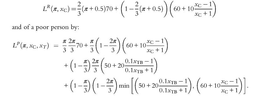
The solution of the program that maximizes the minimum life expectancy of the two types, subject to the budget constraint, is xc = $686, xTB = $13,027. In Figure 4.2, we present the life expectancies of the rich and the poor, as a function of the rank at which they sit on the effort (lifestyle) distribution of their type, at this solution. The higher curve is that of the rich. We see that, at the EOp solution, the rich still have greater life expectancy than the poor—despite the large amounts being spent on treating tuberculosis.[141] The difference, however, is much less than 1 year. Moreover, life expectancy increases with lifestyle quality—this inequality of outcome is an aspect that EOp does not attempt to eliminate.
Let us compare this solution to the utilitarian solution, the expenditure schedule at which life expectancy in the population as a whole is maximized. The solution turns out to be xc = $1915, xTB = $10,571. Three times as much is spent on cancer as in the EOp solution. Figure 4.3 graphs the life expectancy of the two types in the utilitarian solution (dashed lines) as well as the EOp solution (solid lines).
We see that the utilitarian solution narrows the life expectancy differential between the types less than the EOp solution does (although, in absolute terms, the differences are not great in this example). The EOp solution is more egalitarian, across the types, than the
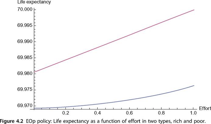
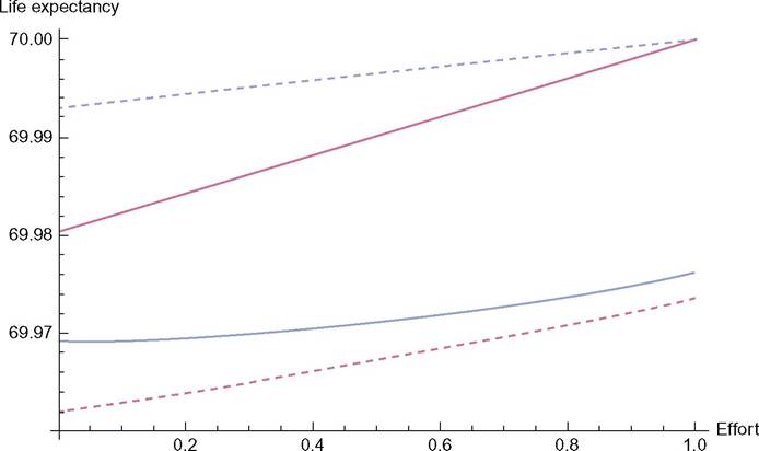
Figure 4.3 Life expectancies of rich and poor, utilitarian (dashed) and EOp (solid) policies.
utilitarian solution—the utilitarian cares only about average life expectancy in aggregate, not on the distribution of life expectancy across types.
It is obvious that different objective functions will engender different optimal solutions. The unfortunate habit that is almost ubiquitous in policy circles is to identify the utilitarian solution with the efficient solution. Critics of the EOp solution will say that it is inefficient because it delivers a lower life expectancy on average for the population than the utilitarian solution. But this is a confusion. Both solutions are Pareto efficient, in the sense that it is impossible, for either of them, to find a policy that weakly increases the life expectancies of everyone. Identifying the utilitarian social objective with efficiency is an unfortunate practice, rooted in the deep hold that utilitarianism has in economics. Social efficiency is defined with respect to whatever the social objective is, and there are many possible choices for that objective besides the social average. We discuss this point with respect to measuring economic development below in Section 4.5.
4.4.