Business Cycle Facts
Describe the behavior of various variables over the course of business cycles.
Although no two business cycles are identical, all (or most) cycles have features in common. This point has been made strongly by a leading business cycle theorist, Nobel laureate Robert E.
Lucas, Jr., of the University of Chicago:Though there is absolutely no theoretical reason to anticipate it, one is led by the facts to conclude that, with respect to the qualitative behavior of comovements among series [that is, economic variables], business cycles are all alike. To theoretically inclined economists, this conclusion should be attractive and challenging, for it suggests the possibility of a unified explanation of business cycles, grounded in the general laws governing market economies, rather than in political or institutional characteristics specific to particular countries or periods.[134]
Lucas's statement that business cycles are all alike (or more accurately, that they have many features in common) is based on examinations of comovements among economic variables over the business cycle. In this section, we study these comovements, which we call business cycle facts, for the post-World War II period in the United States. Knowing these business cycle facts is useful for interpreting economic data and evaluating the state of the economy. In addition, they provide guidance and discipline for developing economic theories of the business cycle. When we discuss alternative theories of the business cycle in Chapters 10 and 11, we evaluate the theories principally by determining how well they account for business cycle facts. To be successful, a theory of the business cycle must explain the cyclical behavior of not just a few variables, such as output and employment, but of a wide range of key economic variables.
The Cyclical Behavior of Economic Variables: Direction and Timing
Two characteristics of the cyclical behavior of macroeconomic variables are important to our discussion of the business cycle facts.
The first is the direction in which a macroeconomic variable moves, relative to the direction of aggregate economic activity. An economic variable that moves in the same direction as aggregate economic activity (up in expansions, down in contractions) is procyclical. A variable that moves in the opposite direction to aggregate economic activity (up in contractions, down in expansions) is countercyclical. Variables that do not display a clear pattern over the business cycle are acyclical.The second characteristic is the timing of the variable's turning points (peaks and troughs) relative to the turning points of the business cycle. An economic variable is a leading variable if it tends to move in advance of aggregate economic activity. In other words, the peaks and troughs in a leading variable occur before the corresponding peaks and troughs in the business cycle. A coincident variable is one whose peaks and troughs occur at about the same time as the corresponding business cycle peaks and troughs. Finally, a lagging variable is one whose peaks and troughs tend to occur later than the corresponding peaks and troughs in the business cycle.
The fact that some economic variables consistently lead the business cycle suggests that they might be used to forecast the future course of the economy. Some analysts have used downturns in the stock market to predict recessions, but such an indicator is not infallible. As Paul Samuelson noted: "Wall Street indexes predicted nine out of the last five recessions."[135]
In some cases, the cyclical timing of a variable is obvious from a graph of its behavior over the course of several business cycles; in other cases, elaborate statistical techniques are needed to determine timing. Conveniently, The Conference Board has analyzed the timing of dozens of economic variables. This information is published monthly in Business Cycle Indicators, along with the most recent data for these variables. For the most part, in this chapter we rely on The Conference Board's timing classifications.
Let's now examine the cyclical behavior of some key macroeconomic variables. We showed the historical behavior of several of these variables in Figs. 1.1-1.4. Those figures covered a long time period and were based on annual data. We can get a better view of short-run cyclical behavior by looking at quarterly or monthly data. The direction and timing of the variables considered are presented in Summary table 10.
Production
Because the level of production is a basic indicator of aggregate economic activity, peaks and troughs in production tend to occur at about the same time as peaks and troughs in aggregate economic activity. Thus production is a coincident and procyclical variable. Figure 8.5 shows the behavior of the industrial production
FIGURE 8.5
Cyclical behavior of the index of industrial production, 1947-2021
The index of industrial production, a broad measure of production in manufacturing, mining, and utilities, is procyclical and coincident.
Source: Board of Governors of the Federal Reserve System, downloaded from Federal Reserve Bank of St. Louis FRED database at fred.stlouisfed. org/series/INDPRO.
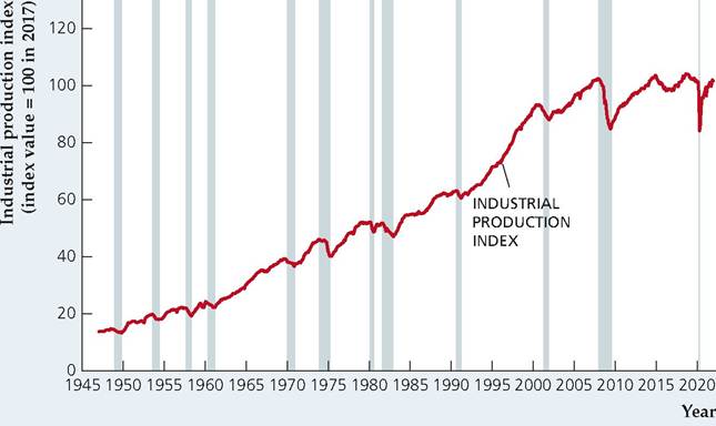
index in the United States since 1947. This index is a broad measure of production in manufacturing, mining, and utilities. The shaded vertical bars in Figs. 8.5-8.13, 8.15, and 8.16 indicate times of recessions, as determined by the NBER (see Table 8.1). The turning points in industrial production correspond closely to the turning points of the cycle.
Although almost all types of production rise in expansions and fall in recessions, the cyclical sensitivity of production in some sectors of the economy is greater than in others. Industries that produce relatively durable, or long-lasting, goods—houses, consumer durables (refrigerators, cars, washing machines), or capital goods (drill presses, computers, factories)—respond strongly to the business cycle, producing at high rates during expansions and at much lower rates during recessions.
In contrast, industries that produce relatively nondurable or short-lived goods (foods, paper products) or services (education, insurance) are less sensitive to the business cycle.SUMMARY 10___________________________________
The Cyclical Behavior of Key Macroeconomic Variables (the Business Cycle Facts)
Variable Direction Timing
Production
Industrial production Procyclical Coincident
Durable goods industries are more volatile than nondurable goods and services
Expenditure
| Consumption | Procyclical | Coincident |
| Business fixed investment | Procyclical | Coincident |
| Residential investment | Procyclical | Leading |
| Inventory investment | Procyclical | Leading |
| Government purchases | Procyclical | __ a |
| Investment is more volatile than consumption | ||
| Labor Market Variables | ||
| Employment | Procyclical | Coincident |
| Unemployment | Countercyclical | Unclassifiedb |
| Average labor productivity | Procyclical | Leadinga |
| Real wage | Procyclical | a |
| Money Supply and Inflation | ||
| Money supply | Procyclical | Leading |
| Inflation | Procyclical | Lagging |
| Financial Variables | ||
| Stock prices | Procyclical | Leading |
| Nominal interest rates | Procyclical | Lagging |
| Real interest rates | Acyclical | a |
aTiming is not designated by The Conference Board.
bDesignated as “unclassified” by The Conference Board; leading at peaks and lagging at troughs.Source: Business Cycle Indicators, April 2018. Industrial production: series 47 (industrial production); consumption: series 57 (manufacturing and trade sales, constant dollars); business fixed investment: series 86 (gross private nonresidential fixed investment); residential investment: series 28 (new private housing units started); inventory investment: series 30 (change in business inventories, constant dollars); employment: series 41 (employees on nonagricultural payrolls); unemployment: series 43 (civilian unemployment rate); money supply: series 106 (money supply M2, constant dollars); inflation: series 120 (CPI for services, change over six-month span); stock prices: series 19 (index of stock prices, 500 common stocks); nominal interest rates: series 119 (Federal funds rate), series 114 (discount rate on new 91-day Treasury bills), series 109 (average prime rate charged by banks).
FIGURE 8.6
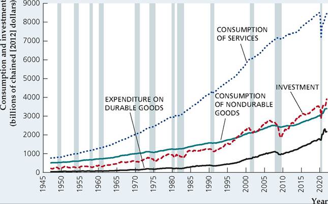
Cyclical behavior of consumption and investment, 1947-2021
Both consumption and investment are procyclical. However, investment is more sensitive than consumption to the business cycle, reflecting the fact that durable goods are a larger part of investment spending than they are of consumption spending. Similarly, expenditures on consumer durables are more sensitive to the business cycle than is consumption of nondurable goods or services.
Source: Authors' calculations based on data from U.S. Bureau of Economic Analysis, downloaded from Federal Reserve Bank of St. Louis FRED database at fred.stlouisfed.org. Durable goods: series DDURRA3Q086SBEA and PCDG; nondurable goods series DNDGRA3Q086SBEA and PCND; services series DSERRA3Q086SBEA and PCESV; investment series GPDIC96.
Expenditure
For components of expenditure, as for types of production, durability is the key to determining sensitivity to the business cycle. Figure 8.6 shows the cyclical behavior of consumption of nondurable goods, consumption of services, consumption expenditures on durable goods, and investment.
Investment is made up primarily of spending on durable goods and is strongly procyclical. In contrast, consumption of nondurable goods and consumption of services are both much smoother. Consumption expenditures on durable goods are more strongly procyclical than consumption expenditures on nondurable goods or consumption of services, but not as procyclical as investment expenditures. With respect to timing, consumption and investment are generally coincident with the business cycle, although individual components of fixed investment vary in their cyclical timing.[136]One component of spending that seems to follow its own rules is inventory investment, or changes in business inventories (not shown), which often displays large fluctuations that aren't associated with business cycle peaks and troughs. In general, however, inventory investment is procyclical and leading. Even though goods kept in inventory need not be durable, inventory investment is also very volatile. Although, on average, inventory investment is a small part (about 1%) of total spending, sharp declines in inventory investment represented a large part of the total decline in spending in some recessions, most notably those of 1973-1975, 1981-1982, and 2001.
Government purchases of goods and services generally are procyclical. Rapid military buildups, as during World War II, the Korean War, and the Vietnam War, are usually associated with economic expansions.
Employment and Unemployment
Business cycles are strongly felt in the labor market. In a recession, employment grows slowly or falls, many workers are laid off, and jobs become more difficult to find.
Figure 8.7 shows the number of civilians employed in the United States since 1955. Employment clearly is procyclical, as more people have jobs in booms than in recessions, and also is coincident with the cycle.
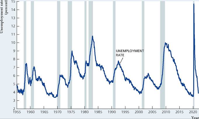
Figure 8.8 shows the civilian unemployment rate, which is the fraction of the civilian labor force (the number of people who are available for work and want to work) that is unemployed. The civilian unemployment rate is strongly countercyclical, rising sharply in contractions but falling more slowly in expansions. Although The Conference Board has studied the timing of unemployment, Summary table 10 shows that the timing of this variable is designated as "unclassified," owing to the absence of a clear pattern in the data. Figures 8.7 and 8.8 illustrate a worrisome change in the patterns of some recessions: namely in most of the recent recessions, employment growth stagnated and unemployment tended to rise for some time even after the recession's trough was reached. This pattern led observers to refer to the recovery periods following these recessions as "jobless recoveries." Fortunately, these recoveries eventually gained strength and the economy showed employment growth and a decline in the rate of unemployment.
FIGURE 8.7
Cyclical behavior of civilian employment, 1955-2021
Civilian employment is procyclical and coincident with the business cycle.
Source: Bureau of Labor Statistics, downloaded from Federal Reserve Bank of St. Louis FRED database at fred.stlouisfed.org/series/CE16OV.
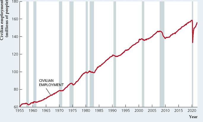
FIGURE 8.8
Cyclical behavior of the unemployment rate, 1955-2021
The unemployment rate is countercyclical and very sensitive to the business cycle. Its timing pattern relative to the cycle is unclassified, meaning that it has no definite tendency to lead, be coincident, or lag.
Source: Bureau of Labor Statistics, downloaded from Federal Reserve Bank of St. Louis FRED database at fred.stlouisfed.org/series/UNRATE.
Application
The Job Finding Rate and the Job Loss Rate
In considering the cyclical movement of employment, we examined the total amount of employment in the economy. As we discussed in Chapter 3, in any given month, we can examine the probability that someone finds a job in that month or loses a job in that month. Those probabilities change over time, depending on whether the economy is in a recession or an expansion. For example, the probability that someone who is unemployed will find a job in the next month, which we call the job finding rate, declines during recessions and increases in expansions. As you might imagine, the probability that someone who is employed will lose their job in the next month, which we call the job loss rate, increases during recessions and decreases in expansions.[137]
Figure 8.9 shows the job finding rate over the course of the business cycle. Notice that the job finding rate generally rises during each economic expansion, and falls in recessions. The decline in recessions is a bit faster than the rise of the job finding rate in expansions. The job finding rate changes substantially over the business cycle. In the expansion of the 1980s, the job finding rate rose from a low of 18% in November 1982 to a peak of 33% in late 1989, an increase of 15 percentage points. In the expansion of the 1990s, the job finding rate rose from 21% in late 1991 to 35% in April 2000, an increase of 14 percentage points. And in
FIGURE 8.9
The job finding rate, 1976-2021
The chart shows monthly data from January 1976 to December 2021 on the rate at which people who are unemployed find new jobs each month, that is, those who report being unemployed one month and employed the next month. The job finding rate rises in expansions and falls in recessions.
Source: Shigeru Fujita and Garey Ramey, “The Cyclicality of Separation and Job Finding Rates,” International Economic Review, May 2009, pp. 415-430; data for January 1976 to January 1990 from Shigeru Fujita and data for February 1990 to December 2021 from Bureau of Labor Statistics website, www.bls.gov/cps/ cps_lows.htm.
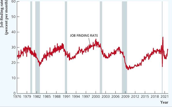
some recessions, such as the one in 2001, the decline in the job finding rate can be sharp, and it sometimes continues to decline even after the recession ends, as occurred following the 1990-1991 recession and the 2001 recession. A particularly disturbing feature of the 2007-2009 recession is the decline of the job finding rate to its lowest point since the data became available in 1976. The job finding rate was slower to rebound in the recovery that began in June 2009 than it did in the three previous recoveries. By mid-2015, 6 years into the recovery, the job finding rate remained well below the levels it reached at the same point in the previous four expansions. By 2018, which is 9 years after the recovery began, the job finding rate finally got back to the level it had been at before the recession.
Figure 8.10 shows the job loss rate, which is the probability that a person employed in one month becomes unemployed the next month.[138] The first thing to notice is that the job loss rate is very low compared with the job finding rate (the scales on Figs. 8.9 and 8.10 are different, so be sure to look at the percentages shown on the vertical axes of both graphs). The job loss rate averaged 1.5% from 1976 to February 2020. It appeared to be on a long steady decline over time in the 1980s and 1990s but did not decline much in the 2000s, and increased sharply in the 2007-2009 recession as well as the COVID recession in 2020. Fortunately, the job loss rate declined in the recovery that began in June 2009, fell below its historical average in October 2011 and continued to decline after that. After the COVID recession the job loss rate plummeted quickly and by 2021 was consistently below its long-run average.
FIGURE 8.10
The job loss rate, 1976-2021
The chart shows monthly data from January 1976 to December 2021 on the rate at which people who are employed lose their jobs each month, that is, those who report being employed one month and unemployed the next month. The job loss rate declines in expansions and rises in recessions.
Source: Same as for Figure 8.9.
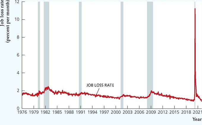
Over the course of the business cycle, the job loss rate generally declines in economic expansions and rises in recessions. Compared with the job finding rate, the changes in the job loss rate are small. So, at first glance, you might think that because the job finding rate falls substantially in recessions, while the job loss rate does not change much, changes in the job finding rate are primarily responsible for changes in the overall unemployment rate for the economy.
To investigate this issue, we will use the data in Table 8.2 to examine job losses and jobs found in an economic expansion and in a recession. First consider changes in employment status during May 2018. As shown in the first column of Table 8.2, in May 2018, the job loss rate was 0.9% and the number of employed workers was 155.3 million, so the number of people who were employed at the start of the month and who became unemployed during the month was 0.009 ? 155.3 million = 1.4 million. Similarly, we can calculate the number of people who were unemployed at the start of the month and who became employed during the month. The job finding rate was 27.1% and the number of unemployed workers was 5.9 million, so the number of people who were unemployed at the start of the month and who became employed during the month was 0.271 ? 5.9 = 1.6 million. With 1.4 million workers losing jobs and 1.6 million workers finding jobs, the number of unemployed people fell by 0.2 million during May 2018.[139]
In a recession, the decline in the job finding rate combined with the rise in the job loss rate together cause the number of employed workers to decline and the number of unemployed workers to rise. For example, consider changes in employment during October 2008, in the middle of the financial crisis. As shown in the second column of
TABLE 8.2
Jobs Lost and Gained In an Expansion and a Recession
| May 2018 (expansion) | October 2008 (recession) | |
| Number of employed people (prior month) | 155.3 million | 145.1 million |
| Job loss rate | 0.9% | 1.6% |
| Number of newly unemployed people | 1.4 million | 2.3 million |
| Number of unemployed people (prior | 5.9 million | 9.5 million |
| month) | ||
| Job finding rate | 27.1% | 22.5% |
| Number of newly employed people | 1.6 million | 2.1 million |
| Net change in number of unemployed | -0.2 million | 0.2 million |
Table 8.2, the job loss rate was 1.6% and the number of employed workers was 145.1 million, so the number of people who were employed at the start of the month and who became unemployed during the month was 0.016 ? 145.1 million = 2.3 million. Similarly, we can calculate the number of people who were unemployed at the start of the month and who became employed during the month. The job finding rate was 22.5% and the number of unemployed workers was 9.5 million, so the number of people who were unemployed at the start of the month and who became employed during the month is 0.225 ? 9.5 million = 2.1 million. With 2.3 million workers losing jobs and only 2.1 million workers finding jobs, the number of unemployed people increased by 0.2 million.
Notice in these calculations that the number of people who are employed is much larger than the number of people who are unemployed. Thus, even though the job finding rate falls by more than the job loss rate rises in recessions, the job loss rate is multiplied by a much larger number than is the job finding rate. For example, during October 2008, the ratio of employed to unemployed was 15 to 1. So, smaller changes in the job loss rate may lead to larger changes in the number of unemployed workers than larger changes in the job finding rate.
In summary, economists have found interesting patterns to the changes in job losses and hiring over the course of the business cycle. The most surprising finding is that the job finding rate declines substantially more than the job loss rate rises during recessions. But since the job loss rate applies to many more people, the increased unemployment that arises during recessions can result as much, or even more, from increased job loss as from decreased job finding.
Average Labor Productivity and the Real Wage
Two other significant labor market variables are average labor productivity and the real wage. As discussed in Chapter 1, average labor productivity is output per unit of labor input. Figure 8.11 shows average labor productivity measured as total real output in the U.S. economy (excluding farms) divided by the total number of hours worked to produce that output. Average labor productivity tends to be procyclical: In booms workers produce more output during each hour of work than they do in recessions.16 Although The Conference Board doesn't designate
16The Application in Chapter 3, “The Production Function of the U.S. Economy and U.S. Productivity Growth,” made the point that total factor productivity A also tends to be procyclical.
FIGURE 8.11
Cyclical behavior of average labor productivity and the real wage, 1955Q1-2021Q4
Average labor productivity, measured as real output per employee hour in the nonfarm business sector, is procyclical and leading. The economywide average real wage is mildly procyclical.
Source: Bureau of Labor Statistics, downloaded from Federal Reserve Bank of St. Louis FRED database at fred.stlouisfed.org series OPHNFB (productivity) and comprnfb (real wage).
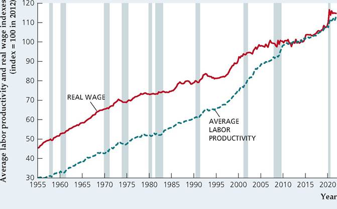
the timing of this variable, studies show that average labor productivity tends to lead the business cycle.[140]
Recall from Chapter 3 that the real wage is the compensation received by workers per unit of time (such as an hour or a week) measured in real, or purchasing-power, terms. The real wage, as shown in Fig. 8.11, is an especially important variable in the study of business cycles because it is one of the main determinants of the amount of labor supplied by workers and demanded by firms. Most of the evidence points to the conclusion that real wages are mildly procyclical, but there is some controversy on this point.[141]
Money Growth and Inflation
Another variable whose cyclical behavior is somewhat controversial is the money supply. Figure 8.12 shows the behavior since 1960 of the growth in the M2 measure of the money supply.[142] Note that (nominal) money growth fluctuates a great
FIGURE 8.12
Cyclical behavior of nominal money growth and inflation, 1960-2021
Nominal money growth, here measured as the six-month moving average of monthly growth rates in M2 (expressed in annual rates), is volatile. However, the figure shows that money growth often falls at or just before a cyclical peak. Statistical and historical studies suggest that, generally, money growth is procyclical and leading. Inflation, here measured as the six-month moving average of monthly growth rates of the personal consumption expenditures price index (expressed in annual rates), is procyclical and lags the business cycle.
Source: Money supply: Board of Governors of the Federal Reserve System, downloaded from Federal Reserve Bank of St. Louis FRED database at fred.stlouisfed.org series M2SL; inflation: Bureau of Labor Statistics, downloaded from FRED database, series PCEPI.
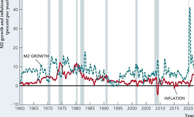
deal and doesn't always display an obvious cyclical pattern. However, as Fig. 8.12 shows, money growth often falls sharply at or just before the onset of a recession. Moreover, many statistical and historical studies—including a classic work by Milton Friedman and Anna J. Schwartz[143] that used data back to 1867—demonstrate that money growth is procyclical and leads the cycle.
The cyclical behavior of inflation, also shown in Fig. 8.12, presents a somewhat clearer picture. Inflation is procyclical but with some lag. Inflation typically builds during an economic expansion, peaks slightly after the business cycle peak, and then falls until some time after the business cycle trough is reached. Atypically, inflation did not increase during the long boom of the 1990s. But inflation did rise substantially in the economic expansions in the 1960s and 1970s. More recently, inflation rose sharply in the aftermath of the COVID recession, following large increases in money-supply growth.
Financial Variables
Financial variables are another class of economic variables that are sensitive to the cycle. For example, stock prices are generally procyclical (stock prices rise in good economic times) and leading (stock prices usually fall in advance of a recession).
Nominal interest rates are procyclical and lagging. The nominal interest rate shown in Figure 8.13 is the rate on three-month Treasury bills. However, other
FIGURE 8.13
Cyclical behavior of the nominal interest rate, 1947-2021
The nominal interest rate, measured here as the interest rate on three- month Treasury bills, is procyclical and lagging. Source: Federal Reserve Board of Governors, downloaded from Federal Reserve Bank of St. Louis FRED database at fred.stlouisfed.org/series/TB3MS.
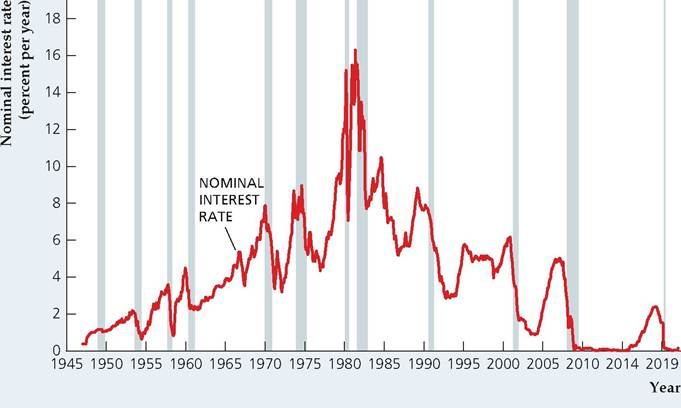
interest rates, such as the prime rate (charged by banks to their best customers) and the Federal funds rate (the interest rate on overnight loans made from one bank to another) also are procyclical and lagging. Note that nominal interest rates have the same general cyclical pattern as inflation; in Chapter 7 we discussed why nominal interest rates tend to move up and down with the inflation rate.
The real interest rate doesn't have an obvious cyclical pattern. For instance, the real interest rate actually was negative during the 1973-1975 recession but was very high during the 1981-1982 recession. (Annual values of the real interest rate are shown in Fig. 2.6.) The acyclicality of the real interest rate doesn't necessarily mean its movements are unimportant over the business cycle. Instead, the lack of a stable cyclical pattern may reflect the facts that individual business cycles have different causes and that these different sources of cycles have different effects on the real interest rate.
International Aspects of the Business Cycle
So far we have concentrated on business cycles in the United States. However, business cycles are by no means unique to the United States, having been regularly observed in all industrialized market economies. In most cases the cyclical behavior of key economic variables in these other economies is similar to that described for the United States.
The business cycle is an international phenomenon in another sense: Frequently, the major industrial economies undergo recessions and expansions at about the same time, suggesting that they share a common cycle. Figure 8.14 illustrates this
FIGURE 8.14
Industrial production indexes in six major countries, 1960-2021 The worldwide effect of business cycles is reflected in the similarity of the behavior of industrial production in each of the six countries shown. But individual countries also have fluctuations not shared with other countries.
Source: OECD Main Economic Indicators, April 2022, downloaded from Federal Reserve Bank of St. Louis FRED database at fred.stlouisfed.org, series GBRPROINDMISMEIf DEUPROINDMISMEIf FRAPROINDMISMEIf JPNPROINDMISMEIf CANPROINDMISMEIf and Usaproindmismei (with scales adjusted for clarity). Note: The scales for the industrial production indexes differ by country; for example, the figure does not imply that the United Kingdom's total industrial production is higher than that of Japan.
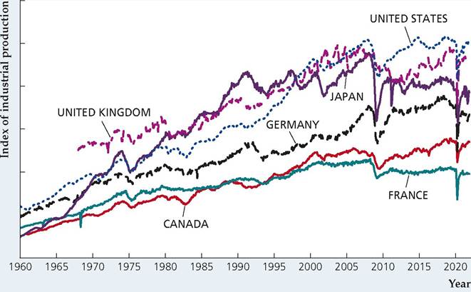
common cycle by showing the index of industrial production since 1960 for each of six major industrial countries. Note in particular the effects of worldwide recessions in about 1975, 1982, 1991, 2001, 2008, and 2020. Figure 8.14 also shows that each economy experiences many small fluctuations not shared by the others.
In Touch with Data and Research
Coincident and Leading Indexes
In this chapter, we discuss a large number of variables and describe how they behave as the economy goes through expansions and contractions. One difficulty faced by policymakers and economic analysts is how to sort through all of the different economic data and figure out where the economy stands overall; a more challenging problem is to forecast, in advance, when the economy will change course. To address these problems, economists have developed coincident and leading indexes. An index is a single number that combines data on a variety of economic variables. A coincident index is an index that is designed to have peaks and troughs that occur about the same time as the corresponding peaks and troughs in aggregate economic activity, and is useful for assessing whether the economy is currently in a recession or an expansion. A leading index is designed to have its peaks and troughs before the corresponding peaks and troughs in aggregate economic activity, and thus might be useful for forecasting turning points in the business cycle.
The first indexes were developed in the 1930s at the NBER by Wesley Mitchell and Arthur Burns,21 whose important early work on business cycles was mentioned earlier in this chapter. Today, these original indexes (with some modification and updating) are produced by The Conference Board, and other indexes have been developed by other economists. In this box, we discuss two recently developed coincident indexes and The Conference Board's index of leading economic indicators.
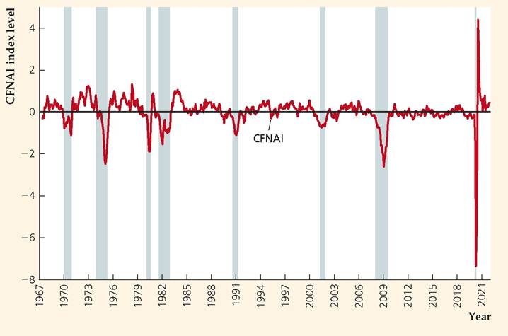
The Chicago Fed National Activity Index (CFNAI) was developed in 2001 by economist Jonas Fisher of the Federal Reserve Bank of Chicago. This coincident index is based on 85 monthly economic variables in five categories: production and income, the labor market, consumption and housing, manufacturing and sales, and inventories and orders. The index is constructed so that it has an average value of 0 over time. Figure 8.15 shows the values of the CFNAI, averaged over the current and preceding two months, since March 1967. The graph includes recession bars, showing the dates of recessions as determined by the NBER. As the graph shows, the CFNAI turns significantly negative in recessions, falling much more in severe recessions (such as 1973-1975, 1981-1982, 2007-2009, and 2020) than in mild recessions (such as 1990-1991 and 2001).[144]
FIGURE 8.15
Chicago Fed National Activity Index, 1967-2021
The chart shows monthly data on the Chicago Fed National Activity Index (CFNAI), averaged over the current and preceding two months. The index tracks recessions closely, falling more in severe recessions than in mild recessions.
Source: Data from Federal Reserve Bank of Chicago, downloaded from Federal Reserve Bank of St. Louis FRED database, fred.stlouisfed.org∕series∕CFNAIMA3.
[1]Statistical Indicators of Cyclical Revivals (New York: National Bureau of Economic Research, 1938).
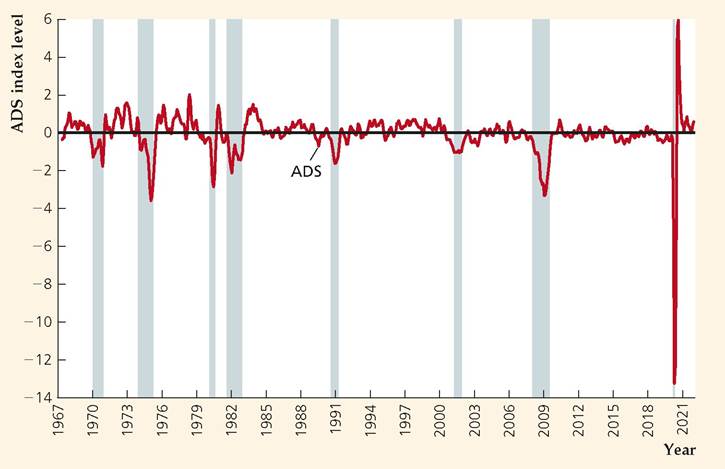
Another recently developed coincident index is the Aruoba-Diebold-Scotti (ADS) Business Conditions Index, which doesn't use as many variables as the CFNAI, but uses variables that have different frequencies: some quarterly data (real GDP), some monthly data (payroll employment, industrial production, personal income less transfer payments, and manufacturing and trade sales), and some weekly data (initial jobless claims). Like the CFNAI, the ADS index is constructed so that it has an average value of 0 over time. The developers of the index, S. Boragan Aruoba of the University of Maryland, Francis X. Diebold of the University of Pennsylvania, and Chiara Scotti of the Federal Reserve Board, sought an index that could be estimated to provide a measure of the state of the economy on a day-by-day basis. They implemented the index in partnership with the Federal Reserve Bank of Philadelphia, which updates the series once or twice each week. Figure 8.16 shows the values of the ADS index, averaged over the current and preceding two months.[145]
Comparing the two indexes, we can see that they are quite similar, despite using very different sets of data. Of course, it is not surprising that the two indexes are similar because they are both designed to measure the underlying state of aggregate economic activity. An advantage of the ADS index is that it is available very frequently (it gets updated once each week or more often). But the CFNAI
[1]For more on the ADS index, see S. Boragan Aruoba, Francis X. Diebold, and Chiara Scotti, “RealTime Measurement of Business Conditions," Journal of Business and Economic Statistics, October 2009, pp. 417-427; the ADS index data are available at the Philadelphia Fed's website at www.philadelphiafed.org/research-and-data/real-time-center/business-conditions-index.
has a longer history of reliability in real time, since it was developed in 2001, whereas the ADS index just began to be produced in real time in 2009.
Unlike the CFNAI and the ADS index, which were designed to measure the current state of the economy, the composite index of leading economic indicators was designed to help anticipate or forecast turning points in aggregate economic activity. However, its record as a forecasting tool is mixed. When the index declines for two or three consecutive months, it warns that a recession is likely. However, its forecasting acumen in real time has not been very good because of the following problems:
1. Data on the components of the index are often revised when more complete data become available. Revisions change the value of the index and may even reverse a signal of a future recession.
2. The index is prone to giving false signals, predicting recessions that did not materialize.
3. The index does not provide any information on when a recession might arrive or how severe it might be.
4. Changes in the structure of the economy over time may cause some variables to become better predictors of the economy and others to become worse. For this reason, the index must be revised periodically, as the list of component indicators is changed.
Research by Francis X. Diebold and Glenn Rudebusch of the Federal Reserve Bank of San Francisco showed that the revisions were substantial.[146] The agency calculating the index (the Commerce Department or The Conference Board) often demonstrates the value of the index with a plot of the index over time, showing how it turns down just before every recession. But Diebold and Rudebusch showed that such a plot is illusory because the index plotted was not the one used at the time of each recession, but rather a revised index made many years after the fact. In real time, they concluded, the use of the index does not improve forecasts of industrial production.
For example, suppose you were examining the changes over time in the composite index of leading indicators, and used the rule of thumb that a decline in the index for three months in a row meant that a recession was likely in the next six months to one year. You would have noticed in December 1969 that the index had declined two months in a row; by January 1970 you would have seen the third monthly decline. In fact, the NBER declared that a recession had begun in December 1969, so the index did not give you any advance warning. Even worse, if you had been following the index in 1973 to 1974, you would have thought all was well until September 1974, when the index declined for the second month in a row, or October 1974, when the third monthly decline occurred. But the NBER declared that a recession had actually begun in November 1973, so the index was nearly a year late in calling the recession.
After missing a recession's onset so badly, the creators of the index naturally want to improve it. So, they may revise the index with different variables, give the variables different weights, or manipulate the statistics so that, if the new revised index had been available, it would have indicated that a recession were coming. For example, the revised index published in April 1979 would have given eight months of lead time before the recession that began in December 1969 and six months of lead time before the recession that began in November 1973. But of course, that index was not available to forecasters when it would have been useful—before the recessions began.
Because of the problems of the official composite index of leading indicators, James Stock and Mark Watson[147] set out to create some new indexes that would improve the value of such indexes in forecasting. They created several experimental leading indexes, with the hope that such indexes would prove better at helping economists forecast turning points in the business cycle. However, it appears that the next two recessions (those that began in 1990 and 2001) were sufficiently different from previous recessions that the experimental leading indexes did not suggest an appreciable probability of recession in either 1990 or 2001. In early 1990, the experimental recession index of Stock and Watson showed that the probability that a recession would occur in the next six months never exceeded 10%. Also, in late 2000 and early 2001, the index did not rise above 10%. So, although the Stock and Watson approach appeared promising in prospect, it did not deliver any improvement in forecasting recessions.
The inability of leading indicators to forecast recessions may simply mean that recessions are often unusual events, caused by large, unpredictable shocks such as disruptions in the world oil supply or a near-collapse of the financial system. If so, then the pursuit of the perfect index of leading indicators may prove to be frustrating.
25"New Indexes of Coincident and Leading Economic Indicators," in Olivier J. Blanchard and Stanley Fischer, eds., NBER Macroeconomics Annual, 1989 (Cambridge, MA: MIT Press, 1989), pp. 351-394.
8.4