Business Cycle Analysis: A Preview

Use aggregate demand and aggregate supply to describe the impact on business cycles of various shocks.

In Touch with Data and Research

The Seasonal Cycle and the Business Cycle

Did you know that GDP in most countries does not consistently grow at the same rate during the various seasons of the year? That may be because macroeconomic data published by governmental statistical agencies are usually seasonally adjusted.

Classic examples of seasonal unemployment are the North African nations of Egypt and Tunisia, which heavily depend on tourism as a major contributor to GDP. Egypt suffers from a seasonal slowdown during the hot summer months, which prevents tourists from visiting a country home to almost 60% of the world's ancient monuments. Conversely, Tunisia is heavily dependent on shore tourism, which dwindles during the colder seasons. In both cases, economic booms are followed by deep recessions. The peak periods of these seasonal cycles account for more than 70% of GDP growth in a country such as Egypt. For the past few decades, economists have attempted to study seasonal fluctuations with the premise that the key variables affecting the business cycle characterize the sea­sonal cycle as well.

One must bear in mind that similar seasonal fluctuations may contribute to the overall business cycle in their own right. These factors must be taken into con­sideration so that government spending becomes procyclical. As discussed later in Chapter 10, classical economists say that business cycles are the best manner by which the economy responds to changes in the economic environment, so macro­economic policy must not eliminate these responses.

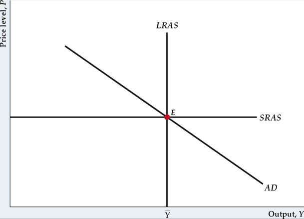
FIGURE 8.17

The aggregate demand-aggregate supply model

The aggregate demand (AD) curve slopes down­ward, reflecting the fact that the aggregate quan­tity of goods and services demanded, Y, falls when the price level, P, rises. The short-run aggregate supply (SRAS) curve is horizontal, reflecting the assumption that, in the short run, prices are fixed and firms simply produce whatever quan­tity is demanded. In the long run, firms produce their normal levels of output, so the long-run aggregate supply (LRAS) curve is vertical at the full-employment level of output, Y. The econo­my's short-run equilib­rium is at the point where the AD and SRAS curves intersect, and its long-run equilibrium is where the AD and LRAS curves intersect.

In general, theories of the business cycle have two main components. The first is a description of the types of factors that have major effects on the economy— wars, new inventions, harvest failures, and changes in government policy are examples. Economists often refer to these (typically unpredictable) forces hitting the economy as shocks. The other component of a business cycle theory is a model of how the economy responds to the various shocks. Think of the economy as a car moving down a poorly maintained highway: The shocks can be thought of as the potholes and bumps in the road; the model describes how the components of the car (its tires and shock absorbers) act to smooth out or amplify the effects of the shocks on the passengers.

The two principal business cycle theories that we discuss in this book are the classical and the Keynesian theories. Fortunately, to present and discuss these two theories we don't have to develop two completely different models. Instead, both can be considered within a general framework called the aggregate demand-aggregate supply, or AD-AS, model. To introduce some of the key differences between the clas­sical and Keynesian approaches to business cycle analysis, in the rest of this chapter we preview the AD-AS model and how it is used to analyze business cycles.

Aggregate Demand and Aggregate Supply: A Brief Introduction

We develop and apply the AD-AS model, and a key building block of the AD-AS model, the IS-LM model, in Chapters 9-11. Here, we simply introduce and briefly explain the basic components of the AD-AS model. The AD-AS model has three components, as illustrated in Figure 8.17: (1) the aggregate demand curve, (2) the short-run aggregate supply curve, and (3) the long-run aggregate supply curve. Each curve represents a relationship between the aggregate price level, P, measured on the vertical axis in Fig. 8.17, and output, Y, measured along the horizontal axis.

The aggregate demand (AD) curve shows for any price level, P, the total quantity of goods and services, Y, demanded by households, firms, and governments, which we call aggregate demand. The AD curve slopes downward in Fig. 8.17, implying that, when the general price level is higher, people demand fewer goods and ser­vices. We give the precise explanation for this downward slope in Chapter 9. The intuitive explanation for the downward slope of the AD curve—that when prices are higher people can afford to buy fewer goods—is not correct. The problem with the intuitive explanation is that, although an increase in the general price level does reflect an increase in the prices of most goods, it also implies an increase in the incomes of the people who produce and sell those goods. Thus to say that a higher price level reduces the quantities of goods and services that people can afford to buy is not correct because their incomes, as well as prices, have gone up.

The AD curve relates the amount of output demanded to the price level, if we hold other economic factors constant. However, for a specific price level, any change in the economy that increases the aggregate quantity of goods and services demanded will shift the AD curve to the right (and any change that decreases the quantity of goods and services demanded will shift the AD curve to the left). For example, a sharp rise in the stock market, by making consumers wealthier, would likely increase households' demand for goods and services, shifting the AD curve to the right. Similarly, the development of more efficient capital goods would increase firms' demand for new capital goods, again shifting the AD curve to the right. Government policies also can affect the AD curve. For example, a decline in government spending on military hardware reduces the aggregate quantity of goods and services demanded and shifts the AD curve to the left.

An aggregate supply curve indicates the amount of output producers are will­ing to supply at any particular price level, which we call aggregate supply. Two aggregate supply curves are shown in Fig. 8.17—one that holds in the short run and one that holds in the long run. The short-run aggregate supply (SRAS) curve, shown in Fig. 8.17, is a horizontal line. The horizontal SRAS curve captures the ideas that in the short run the price level is fixed and that firms are willing to supply any amount of output at that price. If the short run is a very short period of time, such as a day, this assumption is realistic. For instance, an ice cream store posts the price of ice cream in the morning and sells as much ice cream as is demanded at that price (up to its capacity to produce ice cream). During a single day, the owner typically won't raise the price of ice cream if the quantity demanded is unusually high; nor does the owner lower the price of ice cream if the quantity demanded is unusually low. The tendency of a producer to set a price for some time and then supply whatever is demanded at that price is represented by a horizontal SRAS curve.

However, suppose that the quantity of ice cream demanded remains high day after day, to the point that the owner is straining to produce enough ice cream to meet demand. In this case, the owner may raise her price to reduce the quantity of ice cream demanded to a more manageable level. The owner will keep raising the price of ice cream as long as the quantity demanded exceeds normal production capacity. In the long run, the price of ice cream will be whatever it has to be to equate the quantity demanded to the owner's normal level of output. Similarly, in the long run, all other firms in the economy will adjust their prices as necessary so as to be able to produce their normal level of output. As discussed in Chapter 3, the normal level of production for the economy as a whole is called the full-employment level of output, denoted Y.

FIGURE 8.18

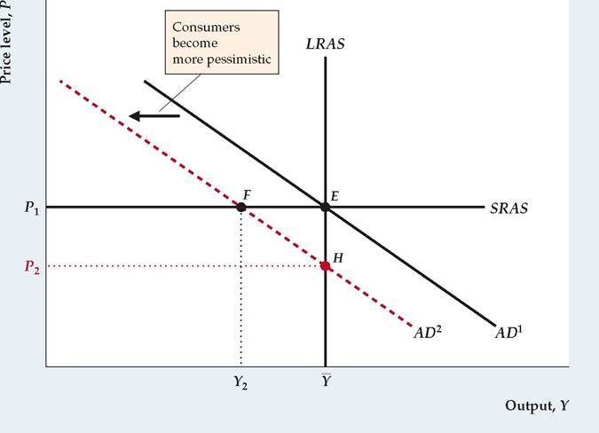
An adverse aggregate demand shock

An adverse aggregate demand shock reduces the aggregate quantity of goods and services demanded at a given price level; an example is that consumers become more pessimistic and thus reduce their spending. This shock is represented by a shift to the left of the aggregate demand curve from AD¹ to AD ². In the short run, the economy moves to point F. At this short-run equilibrium, output has fallen to Y₂ and the price level is unchanged. Eventually, price adjustment causes the economy to move to the new long-run equilibrium at point H, where output returns to its full-employment level, Y, and the price level falls to P₂. In the strict classical view, the economy moves almost immediately to point H, so the adverse aggregate demand shock essentially has no effect on output in both the short run and the long run.

Keynesians argue that the adjustment process takes longer, so that the adverse aggregate demand shock may lead to a sustained decline in output.

output, Y. Thus the long-run aggregate supply (LRAS) curve is vertical, as shown in Fig. 8.17, at the point that output supplied, Y, equals Y.

Figure 8.17 represents an economy that is simultaneously in short-run and long-run equilibrium. The short-run equilibrium is represented by the intersec­tion of the AD and SRAS curves, shown as point E. The long-run equilibrium is represented by the intersection of the AD and LRAS curves, also shown as point E. However, when some change occurs in the economy, the short-run equilibrium can differ from the long-run equilibrium.

Aggregate Demand Shocks. Recall that a theory of business cycles has to include a description of the shocks hitting the economy. The AD-AS framework identifies shocks by their initial effects—on aggregate demand or aggregate supply. An aggregate demand shock is a change in the economy that shifts the AD curve. For example, a negative aggregate demand shock would occur if consumers became more pessimistic about the future and thus reduced their current consumption spending, shifting the AD curve to the left.

To analyze the effect of an aggregate demand shock, let's suppose that the economy initially is in both short-run and long-run equilibrium at point E in Figure 8.18. We assume that, because consumers become more pessimistic, the aggre­gate demand curve shifts down and to the left from AD¹ to AD². In this case, the new short-run equilibrium (the intersection of AD² and SRAS) is at point F, where output has fallen to Y₂ and the price level remains unchanged at P₁. Thus the decline in household consumption demand causes a recession, with output falling below its normal level. However, the economy will not stay at point F forever because firms won't be content to keep producing below their normal capacity. Eventually firms will respond to lower demand by adjusting their prices—in this case downward—until the economy reaches its new long-run equilibrium at point H, the intersection of AD² and LRAS. At point H, output is at its original level, Y, but the price level has fallen to P₂.

Our analysis shows that an adverse aggregate demand shock, which shifts the AD curve down, will cause output to fall in the short run but not in the long run. How long does it take for the economy to reach the long run? This question is cru­cial to economic analysis and is one to which classical economists and Keynesian economists have different answers. Their answers help explain why classicals and Keynesians have different views about the appropriate role of government policy in fighting recessions.

The classical answer is that prices adjust quite rapidly to imbalances in quan­tities supplied and demanded so that the economy gets to its long-run equilibrium quickly—in a few months or less. Thus a recession caused by a downward shift of the AD curve is likely to end rather quickly, as the price level falls and the econ­omy reaches the original level of output Y. In the strictest versions of the classical model, the economy is assumed to reach its long-run equilibrium essentially immediately, implying that the short-run aggregate supply curve is irrelevant and that the economy always operates on the long-run aggregate supply (LRAS) curve. Because the adjustment takes place quickly, classical economists argue that little is gained by the government actively trying to fight recessions. Note that this con­clusion is consistent with the "invisible hand" argument described in Chapter 1, according to which the free market and unconstrained price adjustments are suf­ficient to achieve good economic results.

In contrast to the classical view, Keynesian economists argue that prices (and wages, which are the price of labor) do not necessarily adjust quickly in response to shocks. Hence the return of the economy to its long-run equilibrium may be slow, taking perhaps years rather than months. In other words, although Keynesians agree with classicals that the economy's level of output will eventu­ally return from its recessionary level (represented by Y₂ in Fig. 8.18) to its full­employment level, Y, they believe that this process may be slow. Because they lack confidence in the self-correcting powers of the economy, Keynesians tend to see an important role for the government in fighting recessions. For example, Keynes himself originally argued that government could fight recessions by increasing purchases of goods and services. In terms of Fig. 8.18, an increase in government purchases could in principle shift the AD curve up and to the right, from AD² back to AD¹, restoring the economy to full employment.

Aggregate Supply Shocks. Because classical economists believe that aggre­gate demand shocks don't cause sustained fluctuations in output, they generally view aggregate supply shocks as the major force behind changes in output and employment. An aggregate supply shock is a change in the economy that causes the long-run aggregate supply (LRAS) curve to shift. The position of the LRAS curve depends only on the full-employment level of output, Y, so aggregate supply shocks can also be thought of as factors—such as changes in productivity or labor supply, for example—that lead to changes in Y.

Figure 8.19 illustrates the effects of an adverse supply shock—that is, a shock that reduces the full-employment level of output (an example would be a severe drought that greatly reduces crop yields). Suppose that the economy is initially in long-run equilibrium at point E in Fig. 8.19, where the initial long-run aggregate

FIGURE 8.19

An adverse aggregate supply shock

An adverse aggregate supply shock, such as a drought, reduces the full-employment level of output from Y ι to Y 2. Equivalently, the shock shifts the long-run aggregate supply curve to the left, from LRAS¹ to LRAS². As a result of the adverse supply shock, the long-run equilibrium moves from point E to point F. In the new long-run equilib­rium, output has fallen from Y₁ to Y₂ and the price level has increased from P₁ to P₂.

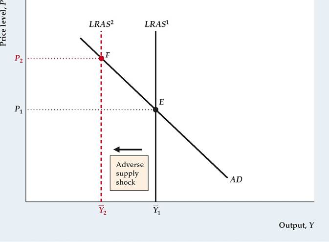
supply curve, LRAS¹, intersects the aggregate demand curve, AD. Now imagine that the adverse supply shock hits, reducing full-employment output from Y₁ to Y₂ and causing the long-run aggregate supply curve to shift to the left from LRAS¹ to LRAS². The new long-run equilibrium occurs at point F, where the level of output is lower than at point E. According to the classical view, the economy moves quickly from point E to point F and then remains at point F. The drop in output as the economy moves from point E to point F is a recession. Note that the new price level, P₂, is higher than the initial price level, P₁, so adverse supply shocks cause prices to rise during recessions. We return to this implication for the price level and discuss its relation to the business cycle facts in Chapter 10.

Although classical economists first emphasized supply shocks, Keynesian economists also recognize the importance of supply shocks in accounting for busi­ness cycle fluctuations in output. Keynesians agree that an adverse supply shock will reduce output and increase the price level in the long run. In Chapter 11, we discuss the Keynesian view of the process by which the economy moves from the short run to the long run in response to a supply shock.

►