Exchange Rates
Describe real and nominal exchange rates, how they are related, and how they change over time.
In discussing exchange rates, we must distinguish between nominal and real exchange rates.
Briefly stated, the nominal exchange rate is the answer to the question: How many units of a foreign currency can I get in exchange for one unit of my domestic currency? The real exchange rate is the answer to the question: How many units of the foreign good can I get in exchange for one unit of my domestic good?Nominal Exchange Rates
Most countries have their own national currencies: The U.S. dollar, the Japanese yen, the British pound, and the Swiss franc are but a few well-known currencies. (Exceptions include a number of European countries, which use the euro as their common currency, and Ecuador, which uses U.S. dollars as its official currency.) If someone in one country wants to buy goods, services, or assets from someone in another country, normally the person buying will first have to trade for the seller's currency to make the payment to complete the transaction.
The rate at which two currencies can be traded is the nominal exchange rate between the two currencies. For example, if the nominal exchange rate between the U.S. dollar and the Japanese yen is 120 yen per dollar, a dollar can buy 120 yen (ignoring transaction costs) in the foreign exchange market, which is the market for international currencies. Equivalently, 120 yen can buy 1 dollar in the foreign exchange market. More precisely, the nominal exchange rate between two currencies, e nom, is the number of units of foreign currency that can be purchased with one unit of the domestic currency. For residents of the United States the domestic currency is the U.S. dollar, and the nominal exchange rate between the U.S. dollar and the Japanese yen is expressed as e nom = 120 yen per dollar.
The nominal exchange rate often is simply called the exchange rate, so whenever someone mentions the exchange rate without specifying real or nominal, the reference is taken to mean the nominal exchange rate.The dollar-yen exchange rate isn't constant. The dollar might trade for 120 yen one day, but the next day it might rise in value to 122 yen or fall in value to 118 yen. Such changes in the exchange rate are normal under a flexible-exchange-rate system, the type of system in which many of the world's major currencies (including the dollar and the yen) are currently traded. In a flexible-exchange-rate system, or floating-exchange-rate system, exchange rates are not officially fixed but are determined by conditions of supply and demand in the foreign exchange market. Under a flexible-exchange-rate system, exchange rates move continuously and respond quickly to any economic or political news that might influence the supplies and demands for various currencies. "In Touch with Data and Research: Exchange Rates," discusses exchange rate data.
The values of currencies haven't always been determined by a flexible-exchangerate system. In the past, some type of fixed-exchange-rate system under which exchange rates were set at officially determined levels, often operated. Usually, these official rates were maintained by the commitment of nations' central banks to buy and sell their own currencies at the fixed exchange rate. For example, under the international gold standard system that operated in the late 1800s and early 1900s, the central bank of each country maintained the value of its currency in terms of gold by agreeing to buy or sell gold in exchange for currency at a fixed rate of exchange. The gold standard was suspended during World War I, was temporarily restored in the late 1920s, and then collapsed during the economic and financial crises of the 1930s.
A more recent example of a fixed-exchange-rate system was the Bretton Woods system, named after the town in New Hampshire where the 1944 conference establishing the system was held.
Under the Bretton Woods system, the values of various currencies were fixed in terms of the U.S. dollar, and the value of the dollar was set at $35 per ounce of gold. The Bretton Woods system functioned until the early 1970s, when inflation in the United States made keeping the price of gold from rising above $35 per ounce virtually impossible. Since the breakdown of the Bretton Woods system, no fixed-exchange-rate system has encompassed all the world's major currencies. In particular, U.S. policymakers haven't attempted to maintain a fixed value for the dollar.Although no worldwide system of fixed exchange rates currently exists, fixed exchange rates haven't disappeared entirely. Many individual countries, especially smaller ones, attempt to fix their exchange rates against a major currency. For example, several African countries tie their currencies to the euro, and from 1991 to 2002, Argentina used a system under which its currency, the peso, traded one-for-one with the U.S. dollar. By fixing their exchange rates, countries hope to stabilize their own currencies and reduce the sharp swings in import and export prices that may result from exchange rate fluctuations. We discuss fixed exchange rates in Section 13.5.
In Touch with Data and Research
Exchange Rates
Exchange rates are determined in foreign exchange markets, in which the currencies of different countries are traded. Principal foreign exchange markets are located in New York, London, Tokyo, and other financial centers. Because foreign exchange markets are in widely separated time zones, at least one of the markets is open at almost any time of the day, so trading in currencies essentially takes place around the clock.
Exchange rates among major currencies often are reported daily on radio and television, and daily quotations of exchange rates are printed in major newspapers and financial dailies. The exchange rates in the accompanying table were reported on the FXEmpire website, wwwfxempire.com/currencies, on May 5, 2022, and apply to transactions on that day.
Three exchange rates relative to the U.S. dollar are reported in the table for each country: a spot rate and two forward rates. All are expressed as units of foreign currency per U.S. dollar. The spot rate is the rate at which foreign currency can be traded immediately for U.S. dollars. For instance, the spot exchange rate for Great Britain, 0.8088, means that on May 5, 2022, one U.S. dollar could buy 0.8088 pounds for immediate delivery.
Forward exchange rates are prices at which you can agree now to buy foreign currency at a specified date in the future. For example, on May 5, 2022, you could have arranged to buy or sell Japanese yen 90 days later at an exchange rate of 130.39 yen per dollar. Note that for the pound and the euro, the 90-day forward exchange rate was lower than the spot exchange rate and the 180-day forward exchange rate was lower than the 90-day forward exchange rate. This pattern of falling forward rates indicates that, as of May 5, 2022, participants in the foreign exchange market expected the value of the dollar relative to the pound and the euro to decrease over the following six months.
Exchange Rate Against U.S. Dollar
| Country | Spot | 90-day forward | 180-day forward |
| Great Britain (pounds per U.S. dollar) | 0.8088 | 0.8083 | 0.8071 |
| Euro Area (euros per U.S. dollar) | 0.9514 | 0.9468 | 0.9407 |
| Japan (yen per U.S. dollar) | 130.39 | 130.39 | 130.38 |
Real Exchange Rates
The nominal exchange rate doesn't tell you all you need to know about the purchasing power of a currency. If you were told, for example, that the nominal exchange rate between the U.S.
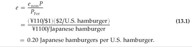
dollar and the Japanese yen is 110 yen per dollar, but you didn't know anything else about the U.S. or Japanese economies, you might be tempted to conclude that someone from Kansas City could visit Tokyo very cheaply—after all, 110 yen for just 1 dollar seems like a good deal. But even at 110 yen per dollar, Japan is an expensive place to visit. The reason is that, although 1 dollar can buy a lot of yen, it also takes a lot of yen (thousands or hundreds of thousands) to buy everyday goods in Japan.Suppose, for example, that you want to compare the price of hamburgers in Tokyo and Kansas City. Knowing that the exchange rate is 110 yen per dollar doesn't help much. But if you also know that a hamburger costs 2 dollars in Kansas City and 1100 yen in Tokyo, you can compare the price of a hamburger in the two cities by asking how many dollars are needed to buy a hamburger in Japan. Because a hamburger costs 1100 yen in Tokyo, and 110 yen cost 1 dollar, the price of a hamburger in Tokyo is 10 dollars (calculated by dividing the price of a Japanese hamburger, ¥1100, by ¥110/$1, to obtain $10 per hamburger). The price of a U.S. hamburger relative to a Japanese hamburger is therefore ($2 per U.S. hamburger ')∕( $10 per Japanese hamburger) = 0.20 Japanese hamburgers per U.S. hamburger. The Japanese hamburger is expensive in the sense that (in this example) one U.S. hamburger equals only one-fifth of a Japanese hamburger.
The price of domestic goods relative to foreign goods—equivalently, the number of foreign goods someone gets in exchange for one domestic good—is called the real exchange rate. In the hamburger example the real exchange rate between the United States and Japan is 0.20 Japanese hamburgers per U.S. hamburger.
In general, the real exchange rate is related to the nominal exchange rate and to prices in both countries. To write this relation we use the following symbols:
e nom = the nominal exchange rate (110 yen per dollar);
PFor = the price of foreign goods, measured in the foreign currency (1100 yen per Japanese hamburger);
P = the price of domestic goods, measured in the domestic currency (2 dollars per U.S.
hamburger).The real exchange rate, e, is the number of foreign goods (Japanese hamburgers) that can be obtained in exchange for one unit of the domestic good (U.S. hamburgers). The general formula for the real exchange rate is
In defining the real exchange rate as the number of foreign goods that can be obtained for each domestic good, we assume that each country produces a single, unique good. (Think of France producing only bottles of wine and Saudi Arabia producing only barrels of oil; then the French real exchange rate with respect to Saudi Arabia is the number of barrels of oil that can be purchased for one bottle of wine.) The assumption that each country produces a single good (which is different from the good produced by any other country) simplifies the theoretical analysis in this chapter.[CCXXXVII]
Of course, in reality, countries produce thousands of different goods, so real exchange rates must be based on price indexes (such as the GDP deflator) to measure P and PFor. Thus the real exchange rate isn't actually the rate of exchange between two specific goods but instead is the rate of exchange between a typical basket of goods in one country and a typical basket of goods in the other country. Changes in the real exchange rate over time indicate that, on average, the goods of the country whose real exchange rate is rising are becoming more expensive relative to the goods of the other country.
Appreciation and Depreciation
When the nominal exchange rate, e nom, falls so that, say, a dollar buys fewer units of foreign currency, we say that the dollar has undergone a nominal depreciation. This is the same as saying that the dollar has become "weaker." If the dollar's nominal exchange rate, e nom, rises, the dollar has had a nominal appreciation. When the dollar appreciates, it can buy more units of foreign currency and thus has become
| SUMMARY 15 | ||
| Terminology for Changes in Exchange Rates | ||
| Type of exchange rate system | Exchange rate increases (currency strengthens) | Exchange rate decreases (currency weakens) |
| Flexible exchange rates | Appreciation | Depreciation |
| Fixed exchange rates | Revaluation | Devaluation |
"stronger."[CCXXXVIII] The terms appreciation and depreciation are associated with flexible exchange rates. Under a fixed-exchange-rate system, in which exchange rates are changed only by official government action, different terms are used. Instead of a depreciation, a weakening of the currency is called a devaluation. A strengthening of the currency under fixed exchange rates is called a revaluation rather than an appreciation. These terms are listed for convenience in Summary table 15.
An increase in the real exchange rate, e, is called a real appreciation. With a real appreciation, the same quantity of domestic goods can be traded for more of the foreign good than before because e, the price of domestic goods relative to the price of foreign goods, has risen. A drop in the real exchange rate, which decreases the quantity of foreign goods that can be purchased with the same quantity of domestic goods, is called a real depreciation.
Purchasing Power Parity
How are nominal exchange rates and real exchange rates related? A simple hypothetical case that allows us to think about this question is when all countries produce the same good (or same set of goods) and goods are freely traded among countries. In this case, no one would trade domestic goods for foreign goods except on a one-for-one basis, so (ignoring transportation costs) the real exchange rate, e, would always equal 1. If e = 1, we can use Eq. (13.1) to write
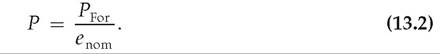
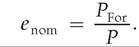
Equation (13.2) says that the price of the domestic good must equal the price of the foreign good when the price of the foreign good is expressed in terms of the domestic currency. (To express the foreign price in terms of the domestic currency, divide by the exchange rate.) The idea that similar foreign and domestic goods, or baskets of goods, should have the same price in terms of the same currency is called purchasing power parity (PPP). Equivalently, as implied by Eq. (13.2), purchasing power parity says that the nominal exchange rate should equal the foreign price level divided by the domestic price level, so that
In Touch with Data and Research
McParity
If PPP holds, similar goods produced in different countries should cost about the same when their prices are expressed in a common currency—say, U.S. dollars. As a test of this hypothesis, The Economist magazine has long recorded the prices of Big Mac hamburgers in different countries. In the table below, the first column of data shows dollar prices of Big Macs in selected countries as reported in The Economist's February 2, 2022, issue.
Big Macs aren't exactly the same product the world over. For example, in Denmark, ketchup costs about 25 cents extra, instead of being included in the price as in the United States and Canada. Nevertheless, the prices suggest that PPP holds only approximately at best for Big Macs. Dollar-equivalent Big Mac prices range from a low of $1.74 in Russia to a high of $6.98 in Switzerland.
Even though PPP fails to hold exactly, Big Mac prices in different countries still might be expected to come gradually closer together. Such a convergence could occur, for example, if the currencies in countries in which Big Macs are relatively expensive depreciated relative to the currencies of the countries in which Big Macs are cheap. Such a calculation would suggest that the Swiss franc is likely to depreciate in value relative to the dollar (because Big Macs are most expensive there). In contrast, the Big Mac index suggests that all of the other currencies shown in the table may appreciate against the dollar. Even though an undervalued currency may appreciate, we don't know when it might appreciate. It could take a number of years for the currency to appreciate, so forecasting movements in exchange rates based on PPP is difficult at best.
Big Mac Prices Around the World
| Dollar price | GDP adjusted | |
| United States | $5.81 | 0% |
| Argentina | 4.29 | 20 |
| Brazil | 4.31 | 23 |
| Canada | 5.32 | 7 |
| China | 3.83 | 5 |
| Euro area | 4.95 | 4 |
| Great Britain | 4.82 | -1 |
| India | 2.55 | -23 |
| Japan | 3.38 | -30 |
| Mexico | 3.34 | -6 |
| Russia | 1.74 | -52 |
| South Korea | 3.82 | -16 |
| Switzerland | 6.98 | 3 |
Source: The Economist magazine, www.economist.com/big-mac-index
With only one country's dollar price above the U.S. price, is something incorrect about the theory of purchasing power parity? Many economists now believe the PPP theory is not very useful and have worked on other versions of the theory. One version, now used by The Economist magazine in its comparison of Big Mac prices, is that the wages paid to workers who produce Big Macs in different countries are directly related to each country's GDP per capita. As a result, Big Mac prices are higher in countries with higher real GDP per capita. The data confirm that result.
So The Economist now also shows the percentage deviations of a country's Big Mac dollar price after adjusting for differences in GDP per capita.3 In the table, these percentage deviations are shown in the column headed "GDP adjusted."
The results show that once an adjustment for GDP per capita is made, about half of the countries have a Big Mac price that is higher than expected, and the other half have a Big Mac price that is lower than expected. After making this adjustment, the Big Mac price in Switzerland, which was the only country with a dollar price higher than the U.S. price, is only 3% higher than expected, whereas the price in Brazil is 23% higher than expected. The lowest adjusted price is Russia, at 52% less than expected. So, this alternative view of PPP seems to fit the data a bit better than the original PPP theory does.
3Formatly, this is done by running an econometric regression of Big Mac dollar prices for each country on the country's real GDP per capita and then calculating the residual. There is some empirical evidence that PPP holds in the very long run, but (as "In Touch with Data and Research: McParity" suggests) over shorter periods PPP does not describe exchange rate behavior very well. The failure of PPP in the short to medium run occurs for various reasons. For example, countries produce different baskets of goods and services, not the same goods as assumed for PPP; some types of goods and services are not internationally traded; and transportation costs and legal barriers to trade may prevent the prices of traded goods and services from being equalized in different countries.
To find a relationship between real and nominal exchange rates that holds more generally, we can use the definition of the real exchange rate in Eq. (13.1), e = e nomP/PFor, to calculate ∆e∕e, the percentage change in the real exchange rate. Because the real exchange rate is expressed as a ratio, its percentage change equals the percentage change in the numerator minus the percentage change in the denominator.4 The percentage change in the numerator of the expression for the real exchange rate5 is ∆e nom∣ e nom + ∆P∣P, and the percentage change in the denominator is ΔPfoJPFor. Thus the percentage change in the real exchange rate is 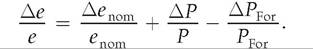
In the preceding equation the term ∆P∣P, the percentage change in the domestic price level, is the same as the domestic rate of inflation, π, and the term ΔPfoi∕PFor, the percentage change in the foreign price level, is the same as the foreign rate of inflation, π For. Making these substitutions and rearranging the equation, we rewrite this equation as 

4Appendix A, Section A.7, describes how to calculate growth rates of products and ratios.
5This result is obtained by using the rule that the percentage change in a product XY is the percentage change in X plus the percentage change in Y. See Appendix A, Section A.7.
rate of real exchange rate appreciation, ∆e∕e, plus the excess of foreign inflation over domestic inflation, π For — π. Hence two factors contribute to strengthening a currency (a nominal appreciation): (1) an increase in the relative price of a country's exports (a real appreciation), which might occur if, for example, foreign demand for those exports rises; and (2) a rate of domestic inflation, π, lower than that of the country's trading partners, π For.
A special case of Eq. (13.3) occurs when the real exchange rate is constant, so that
In this case, the preceding equation expresses a relationship called relative purchasing power parity. According to relative purchasing power parity, the rate of appreciation of the nominal exchange rate equals the foreign inflation rate minus the domestic inflation rate. Relative purchasing power parity usually works well for high-inflation countries because in those countries, differences in relative inflation rates are usually much larger than changes in the real exchange rate.
The Real Exchange Rate and Net Exports
We've defined the real exchange rate, but so far we haven't indicated why it is important in macroeconomic analysis. One reason that policymakers and the public care about the real exchange rate is that it represents the rate at which domestic goods and services can be traded for those produced abroad. An increase in the real exchange rate—also sometimes referred to as the terms of trade—is good for a country in the sense that its citizens are able to obtain more foreign goods and services in exchange for a given amount of domestic production.
A second reason is that the real exchange rate affects a country's net exports, or exports less imports. Changes in net exports in turn have a direct impact on the domestic industries that produce for export or that compete with imported goods in the domestic market. In addition, as we discuss later in the chapter, changes in net exports affect a country's overall level of economic activity and are a primary channel through which business cycle disturbances and macroeconomic policy changes are transmitted internationally.
What is the link between the real exchange rate and net exports? A basic determinant of the demand for any good or service—say, coffee or taxi rides—is the price of that good or service relative to alternatives. If the price of coffee is too high, some people will switch to tea; if taxi fares rise, more people will take the bus. Similarly, the real exchange rate—the price of domestic goods relative to foreign goods—helps determine the demand for domestic goods both in home and foreign markets.
Suppose that the real exchange rate is high, so that a unit of the domestic good can buy relatively many units of the foreign good. For example, let's say that a domestically produced car costs twice as much as a comparable foreign car (both prices are measured in terms of the same currency). Domestic residents will then find that foreign cars are less expensive than domestic cars, so (all else being equal) their demand for imported autos will be high. Foreign residents, in contrast, will find that the domestic country's cars are more expensive than their own, so they will want to purchase relatively few of the domestic country's exports. With few cars being sold abroad and many cars being imported, the country's net exports of cars will be low, probably even negative.
Conversely, suppose that the real exchange rate is low; for example, imagine that a domestically produced automobile costs only half what a comparable foreign car costs. Then, all else being equal, the domestic country will be able to export relatively large quantities of cars and will import relatively few, so that its net exports of cars will be high.
The general conclusion, then, is that the higher the real exchange rate is, the lower a country's net exports will be, holding constant other factors affecting export and import demand. The reason for this result is the same reason that higher prices reduce the amount of coffee people drink or the number of taxi rides they take. Because the real exchange rate is the relative price of a country's goods and services, an increase in the real exchange rate induces both foreigners and domestic residents to consume less domestic production and more goods and services produced abroad, which lowers net exports.
The J Curve. Although the conclusion that (holding other factors constant) a higher real exchange rate depresses net exports is generally valid, there is one important qualification: Depending on how quickly importers and exporters respond to changes in relative prices, the effect of a change in the real exchange rate on net exports may be weak in the short run and may even go the "wrong" way.
To understand why, consider a country that imports most of its oil and suddenly faces a sharp increase in world oil prices. Because the country's domestic goods now can buy less of the foreign good (oil), the country's real exchange rate has fallen. In the long run, this decline in the real exchange rate may increase the country's net exports because high oil prices will lead domestic residents to reduce oil imports and the relative cheapness of domestic goods will stimulate exports (to oil-producing countries, for example). In the short run, however, switching to other fuels and increasing domestic oil production are difficult, so the number of barrels of oil imported may drop only slightly. For this reason, and because the real cost of each barrel of oil (in terms of the domestic good) has risen, for some period of time after the oil price increase the country's total real cost of imports (measured in terms of the domestic good) may rise. Thus in the short run, a decline in the real exchange rate might be associated with a drop rather than a rise in net exports, contrary to our earlier conclusion. (Numerical Problem 2 at the end of the chapter provides an example of how a real depreciation can cause net exports to fall.)
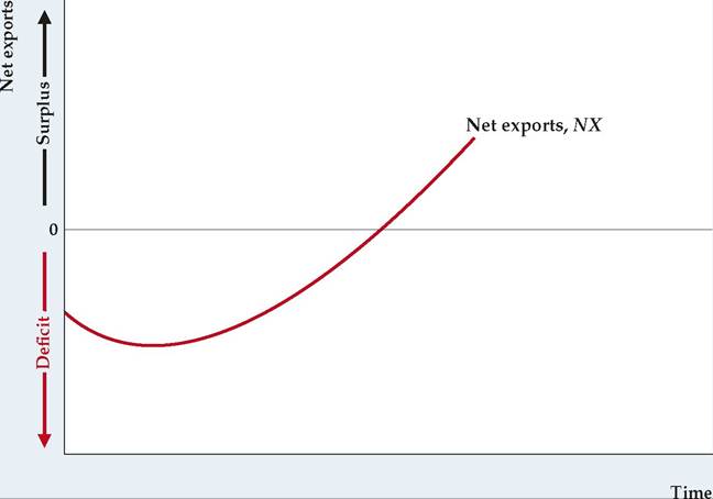
Figure 13.1 shows the typical response pattern of a country's net exports to a drop in the real exchange rate (a real depreciation). The economy initially has negative net exports when the real exchange rate depreciates. In the short run, the real depreciation reduces rather than increases net exports because the drop in the real exchange rate forces the country to pay more for its imports. Over time, however, as the lower real exchange rate leads to larger export quantities and smaller import quantities, net exports begin to rise (even taking into account the higher relative cost of imports). Eventually, the country's net exports rise relative to the initial situation. This typical response pattern of net exports to a real depreciation is called the J curve because the graph of net exports against time looks like the letter J lying on its back.
The macroeconomic analyses in this chapter are based on the assumption that the time period is long enough that (all else being equal) a real depreciation increases net exports and that a real appreciation reduces net exports. Keep in mind, though, that this assumption may not be valid for shorter periods—and in some cases, even for several years—as the following application demonstrates.
FIGUREJ3.1
The J curve
The J curve shows the response pattern of net exports to a real depreciation. Here, net exports are negative at time zero, when the real exchange rate depreciates. In the short run, net exports become more negative, as the decline in the real exchange rate raises the real cost of imports (measured in terms of the export good). Over time, however, increased exports and reduced quantities of imports more than compensate for the increased cost of imports, and net exports rise above their initial level.
Application
The Value of the Dollar and U.S. Net Exports
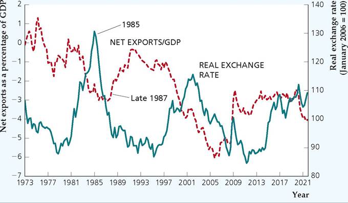
In the early 1970s, the major industrialized countries of the world switched from fixed to flexible exchange rates. Figure 13.2 shows the U.S. real exchange rate (the "real value of the dollar") and real U.S. net exports since 1973. Because the U.S. real exchange rate is the relative price of U.S. goods, the real value of the dollar and U.S. net exports should move in opposite directions (assuming that changes in the real exchange rate are the primary source of changes in net exports).
An apparent confirmation that the real exchange rate and net exports move in opposite directions occurred during the early 1980s. From 1980 to 1985, the real value of the dollar increased by about 50%. This sharp increase was followed, with a brief delay, by a large decline in U.S. net exports. At the time, many U.S. firms complained that the strong dollar was pricing their products out of foreign markets and, by making imported goods cheap for U.S. consumers, also reducing their sales at home.
After peaking in March 1985, the real value of the dollar fell sharply for almost three years. Despite this precipitous decline, U.S. net exports continued to fall until late in 1987, when they finally began to rise. During the two and a half years in which U.S. net exports continued to decline despite the rapid depreciation of the dollar, the public and policymakers expressed increasing skepticism about economists' predictions that the depreciation would lead to more net exports. Initially, economists responded by saying that, because of the J curve, there would be some delay between the depreciation of the dollar and the improvement in net exports. By 1987, however, even the strongest believers in the J curve had begun to wonder whether net exports would ever begin to rise. Finally, U.S. real net exports did recover substantially, although they remained negative.
FIGUREJ3.2
U.S. net exports as a percentage of GDP and the real exchange rate, 1973Q1-2021Q4 U.S. net exports as a percentage of GDP from the first quarter of 1973 to the fourth quarter of 2021 are measured along the left vertical axis, and the U.S. real exchange rate (the real value of the dollar) is measured along the right vertical axis. The sharp increase in the real exchange rate in the first half of the 1980s was accompanied by a decline in U.S. net exports. The decline of the dollar after 1985 stimulated U.S. net exports, but with a delay that probably reflected the J-curve effect.
Sources: Real exchange rate: U.S. real broad dollar index, Federal Reserve Board of Governors, downloaded from Federal Reserve Bank of St. Louis FRED database, fred.stlouisfed.org, series TWEXBPA and RTWEXBGS, spliced together at 2006Q1; net exports as a percentage of GDP, from FRED database, series NETEXP and GDP.
What took so long? One explanation suggests that, because the dollar was so strong in the first half of the 1980s (which made U.S. goods very expensive relative to foreign goods), U.S. firms lost many of their foreign customers. Once these foreign customers were lost, regaining them or adding new foreign customers was difficult, especially as many U.S. exporters reduced production capacity and cut back foreign sales operations when the value of the dollar was high. Similarly, the strong dollar gave foreign producers, including some that hadn't previously sold their output to the United States, a chance to make inroads into the U.S. domestic market. Having established sales networks and customer relationships in the United States, these foreign companies were better able than before to compete with U.S. firms when the dollar began its decline in 1985. The idea that the strong dollar permanently increased the penetration of the U.S. market by foreign producers, while similarly reducing the capability of U.S. firms to sell in foreign markets, has been called the "beachhead effect."[239]
The U.S. real exchange rate and U.S. net exports moved in opposite directions again from 1997 to 2001, as the dollar strengthened and net exports fell sharply. In part this decline in net exports reflected the higher value of the dollar. However, the major factor in this episode was probably the slow growth or outright recession experienced by most U.S. trading partners during this period. As incomes abroad stagnated or declined, the demand for U.S. exports fell with them. We discuss the effects of national income on imports and exports in the next section.
After reaching a peak in early 2002, the dollar weakened for the next six years. It took some time for net exports relative to GDP to reverse course and begin rising, but this ratio finally began to rise in 2006 and continued doing so until 2008. Then, in the financial crisis of 2008, investors' loss of confidence throughout the world led them to buy dollar-denominated assets for safety, causing the dollar to appreciate sharply. At the same time, the fall in U.S. income caused imports
to decline sharply—by more than the decline in foreign income reduced U.S. exports—so that U.S. net exports increased. Following the crisis, the dollar resumed its long-term decline and the ratio of net exports to GDP fell somewhat, but remained well above its level before the crisis. Then, in 2014, the dollar began to appreciate sharply, as the U.S. Federal Reserve ended its quantitative easing program, and central banks in Europe and Japan began large quantitative easing programs (reducing their long-term interest rates and leading investors to purchase more dollar-denominated assets), which we discuss in more detail in Chapter 14.
13.2
More on the topic Exchange Rates:
- English Monetary Theories and Debates in the Age of Classical Economics
- Oman
- Abel A.B., Bernanke B., Croushore D.. Macroeconomics. 10th Edition, Global Edition. — Pearson,2021. — 690 pp., 2021
- The Business Cycle and Economic Policy
- The Theory of Capital
- Bahrain
- Zimbabwe Village Savings and Loan Associations
- References
- Violence in the Mesolithic