Exercises

EXERCISE 10.1. Formulate, state and prove the Separation Theorem, Theorem 10.1, in an economy in discrete time.

Exercise 10.2. (1) Consider the environment discussed in Section 10.1.

budget constraint of the individual as

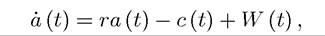
and suppose that there are credit market imperfections so that a (t) ≥ 0. Construct an example in which Theorem 10.1 does not apply. Can you generalize this to the case in which the individual can save at the rate r, but can only borrow at the rate Ã^{0 r}ff ?

(2) Now modify the environment so that the instantaneous utility function of the indi­vidual is

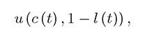
where l (t) denotes total hours of work, labor supply at the market is equal to l (t) — s (t), so that the individual has a non-trivial leisure choice. Construct an example in which Theorem 10.1 does not apply.

Exercise 10.3. Derive equation (10.9) from (10.8).

EXERCISE 10.4. Consider the model presented in Section 10.2 and suppose that the discount rate r varies across individuals (for example, because of credit market imperfections). Show that individuals facing a higher r would choose lower levels of schooling. What would happen if you estimate the wage regression similar to (10.12) in a world in which the source of difference in schooling is differences in discount rates across individuals?

EXERCISE 10.5. Consider the following variant of the Ben-Porath model, where the human capital accumulation equation is given by

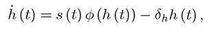
where φ is strictly increasing, continuously differentiable and strictly concave, with s (t) ∈ [0,1].

of u > 0. Show that the optimal path of human capital investments involves s (t) = 1 for some interval [0,T] and then s (t) = s* for t ≥ T.

Exercise 10.6. Modify the Ben-Porath model studied in Section 10.3 as follows. First, assume that the horizon is finite. Second, suppose that φ⁰ (0) < ∞. Finally, suppose that lim_x→h(o) φ⁰ (x) > 0. Show that under these conditions the optimal path of human capital accumulation will involve an interval of full-time schooling with s (t) = 1, followed by another interval of on-the-job investment s (t) ∈ (0,1), and finally an interval of no human capital investment, s (t) = 0. How do the earnings of the individual evolve over the life cycle?

Exercise 10.7. Prove that as long as Y (t) = F (K (t),H (t)) satisfies Assumptions 1 and 2, the inequality in (10.29) holds.

Exercise 10.8. Show that equilibrium dynamics in Section 10.5 remain unchanged if δ < 1. Exercise 10.9. Prove that the current-value Hamiltonian in (10.23) is jointly concave in (k (t),h (t),i_k (t),i_h (t)).

Exercise 10.10. Prove that (10.24) implies the existence of a relationship between physical and human capital of the form h = ξ (k), where ξ (∙) is uniquely defined, strictly increasing and continuously differentiable.

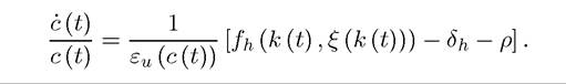
Exercise 10.11. Prove 10.1. Show that the differential equation for consumption growth could have alternatively been written as

Exercise 10.12. Consider the neoclassical growth model with physical and human capital discussed in Section 10.4.

(1) Specify the consumer maximization problem in this economy.

(2) Define a competitive equilibrium (specifying firm optimization and market clearing conditions).

(3) Characterize the competitive equilibrium and show that it coincides with the solution to the optimal growth problem.

Exercise 10.13. Introduce labor-augmenting technological progress at the rate g into the neoclassical growth model with physical and human capital discussed in Section 10.4.

(1) Define a competitive equilibrium.

(2) Determine transformed variables that will remain constant in a steady state alloca­tion.

(3) Characterize the steady state equilibrium and the transitional dynamics.

(4) Why does faster technological progress lead to more rapid accumulation of human capital?

Exercise 10.14. * Characterize the optimal growth path of the economy in Section 10.4 subject to the additional constraints that i⅛ (t) ≥ 0 and ih (t) ≥ 0.

Exercise 10.15. Derive equation (10.25).

Exercise 10.16. Derive equations (10.32) and (10.33).

Exercise 10.17. Provide conditions on f (∙) and γ (∙) such that the unique steady-state equilibrium in the model of Section 10.5 is locally stable.

Exercise 10.18. Analyze the economy in Section 10.6 under the closed economy assumption. Show that an increase in ai for group 1 will now create a dynamic externality, in the sense that current output will increase and this will lead to greater physical and human capital investments next periods.

Exercise 10.19. Prove Proposition 10.5.