Exercises

EXERCISE 6.1. Consider the formulation of the discrete-time optimal growth model as in Example 6.1. Show that with this formulation and Assumptions 1 and 2 from Chapter 2, the discrete-time optimal growth model satisfies Assumptions 6.1-6.5.

Exercise 6.2. * Prove that if for some n ∈ N Tⁿ is a contraction over a complete metric space (S, d), then T has a unique fixed point in S.

Exercise 6.3. * Suppose that T is a contraction over the metric space (S, d) with modulus β ∈ (0,1). Prove that for any z,z⁰ ∈ S and n ∈ N,

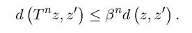
Discuss how this result can be useful in numerical computations.

Exercise 6.4. *

(1) Prove the claims made in Example 6.3 and show that the differential equation in (6.7) has a unique continuous solution.

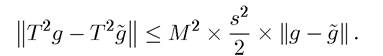
(2) Recall eq. (6.8) from Example 6.3. Now apply the same argument to Tg and Tg and prove that

(3) Applying this argument recursively, prove that for any n ∈ N, we have

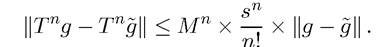
(4) Using the previous inequality, the fact that for any B < ∞, Bⁿ/n! → 0 as n → 0 and the result in Exercise 6.2, prove that the differential equationin (6.7) has a unique continuous solution on the compact interval [0,s] for any

Exercise 6.5. * Recall the Implicit Function Theorem, Theorem A.26 in Appendix Chapter A. Here is a slightly simplified version of it: consider the function φ (y,x) such that that φ : R? [a,b] → R is continuously differentiable with bounded first derivatives.

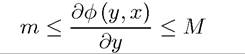
for all x and y. Then, the Implicit Function Theorem states that there exists a continuously differentiable function y : [a,b] → R such that

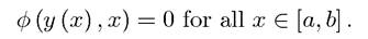
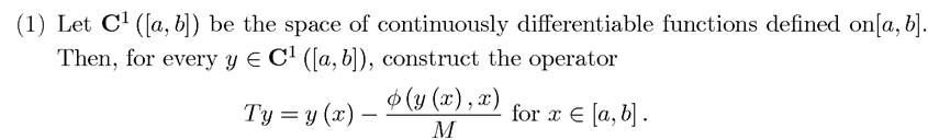
Provide a proof for this theorem using the Contraction Mapping Theorem, Theorem 6.7 along the following lines:

248

Show that T : C¹ ([a, b]) → C¹ ([a, b]) and is a contraction.

(2) Applying Theorem 6.7 derive the Implicit Function Theorem.

Exercise 6.6. * Prove that T defined in (6.18) is a contraction.

Exercise 6.7. Let us return to Example 6.4.

(1) Prove that the law of motion of capital stock given by (6.34) monotonically converges to a unique steady state value of k* starting with any ko > 0. What happens to the level of consumption along the transition path?

(2) Now suppose that instead of (6.34), you hypothesize that

π (x) = ax^α + bx + c.

Verify that the same steps will lead to the conclusion that b = c = 0 and a = βa.

(3) Now let us characterize the explicit solution by guessing and verifying the form of the value function. In particular, make the following guess: V (x) = A lnx, and using this together with the first-order conditions derive the explicit form solution.

Exercise 6.8. Consider the following discrete-time optimal growth model with full depreci­ation:

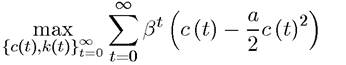
subject to

k (t + 1) = Ak (t) — c (t)

and k (0) = ko. Assume that k (t) ∈ [0, and a < /c^-1, so that the utility function is always

increasing in consumption.

(1) Formulate this maximization problem as a dynamic programming problem.

(2) Argue without solving this problem that there will exist a unique value function V (k) and a unique policy rule c = π (k) determining the level of consumption as a function of the level of capital stock.

(3) Solve explicitly for V (k) and π (k) [Hint: guess the form of the value function V (k), and use this together with the Bellman and Euler equations; verify that this guess satisfies these equations, and argue that this must be the unique solution].

Exercise 6.9. Consider Problem Al or A2 with x ∈ X ⊂ R and suppose that Assumptions 6.1-6.3 and 6.5 hold and that ∂²U (x,y) /∂x∂y ≥ 0. Show that the optimal policy function y = π (x) is nondecreasing.

Exercise 6.10. Show that in Theorem 6.10, a sequencethat satisfies the Euler

equations, but not the transversality condition could yield a suboptimal plan.

Exercise 6.11. Consider the consumer utility maximization problem in Example 6.5, with­out the borrowing limits (that is, only with the flow budget constraint). Show that for any path of consumptionthat satisfies the flow budget constraint starting with an ini­tial asset level a (0), so does the path of consumptionwherefor

7 > 0. Using this result, show that the consumer can reach infinite utility by choosing a 249

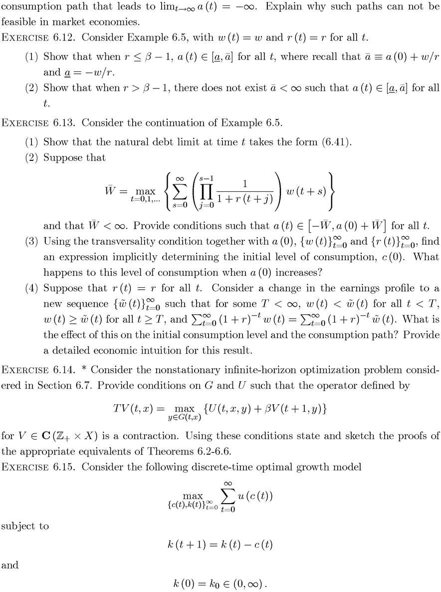
Assume that u (∙) is a strictly increasing, strictly concave and bounded function. Prove that there exists no optimal solution to this problem. Explain why.

Exercise 6.16. Consider the following discrete-time optimal growth model with full depre-

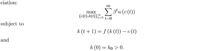
Assume that u (∙) is strictly concave and increasing for c ≥ 0, and f (∙) is concave and increasing.

(1) Formulate this maximization problem as a dynamic programming problem.

(2) Prove that there exists unique value function V (k) and a unique policy rule c = π (k), and that V (k) is continuous and strictly concave and π (k) is continuous and increasing.

(3) When will V (k) be differentiable?

(4) Assuming that V (k) and all the other functions are differentiable, characterize the Euler equation that determines the optimal path of consumption and capital accu­mulation.

(5) Is this Euler equation enough to determine the path of k and c? If not, what other condition do we need to impose? Write down this condition and explain intuitively why it makes sense.