Government Deficits and Debt

Discuss the economic effects of government deficits and debt.

The single number in the Federal government's budget that is the focus of most public attention is the size of the budget deficit or surplus.

The Growth of the Government Debt

There is an important distinction between the government budget deficit and the government debt (also called the national debt). The government budget deficit (a flow variable) is the difference between expenditures and tax revenues in any fiscal year. The government debt (a stock variable) is the total value of govern­ment bonds outstanding at any particular time. Because the excess of government expenditures over revenues equals the amount of new borrowing that the govern­ment must do—that is, the amount of new government debt that it must issue— any year's deficit (measured in dollar, or nominal, terms) equals the change in the debt in that year. We can express the relationship between government debt and the budget deficit by

∆B = nominal government budget deficit, (15.3)

where ∆B is the change in the nominal value of government bonds outstanding.

In a period of persistently large budget deficits, such as that experienced by the United States in the 1980s and early and mid-1990s, and again after 2002, the nominal value of the government's debt will grow quickly. For example, between 1980 and 2021, Federal government debt held by the public grew by over 30 times

¹³David Bizer and Steven Durlauf, “Testing the Positive Theory of Government Finance,” Journal of Monetary Economics, August 1990, pp.

FIGUREJ5.7

Ratio of Federal debt to GDP, 1939-2021 The upper curve shows the ratio of total govern­ment debt—including government bonds held by government agencies and the Federal

Reserve—to GDP. The lower curve shows the ratio of government bonds held by the public to GDP. The debt-GDP ratio rose dramatically during World War II, fell steadily for the next 35 years, and then rose again from 1980 until the mid-1990s. The surpluses of the late 1990s reduced the debt-GDP ratio con­siderably, though large deficits beginning in 2002 increased this ratio.

Source: Economic Report of the President, downloaded from Federal Reserve Bank of St. Louis FRED database, vari­ables FYGFDPUB (publicly held debt), FYGFD (gross debt), GDP (GDP).

in nominal terms, from $712 billion in 1980 to $22,284 billion in 2021.^[290] Taking inflation into account, the real value of government debt outstanding increased more than 11-fold during this period.

Because countries with a high GDP have relatively more resources available to pay the principal and interest on the government's bonds, a useful measure of government indebtedness is the quantity of government debt outstanding divided by the GDP, or the debt-GDP ratio. Figure 15.7 shows the history of the debt-GDP ratio in the United States since 1939. The upper curve shows the debt-GDP ratio when the measure of total government debt outstanding includes both government bonds held by the public and government bonds held by government agencies and the Federal Reserve. The lower curve includes in the measure of debt outstanding only the government debt held by the public, which, strictly speaking, includes the Federal Reserve.

The most striking feature of Fig. 15.7 is the large increase in the debt-GDP ratio that occurred during World War II when the government sold bonds to finance the war effort. By the end of the war, the debt-GDP ratio exceeded 100%, implying that the value of government debt outstanding was greater than a year 's GDP.

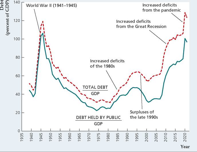
We can describe changes in the debt-GDP ratio over time by the following formula (derived in Appendix 15. A at the end of the chapter):

Equation (15.4) emphasizes two factors that cause the debt-GDP ratio to rise quickly:

■ a high deficit relative to GDP and

■ a slow rate of GDP growth.

Equation (15.4) helps account for the pattern of the debt-GDP ratio shown in Fig. 15.7. The sharp increase during World War II was the result of large deficits. In contrast, for the three and a half decades after World War II, the Federal govern­ment's deficit was small and GDP growth was rapid, so the debt-GDP ratio declined. The debt-GDP ratio increased during the 1980s and early 1990s because the Federal deficit was high. Large surpluses helped reduce the debt-GDP ratio in the late 1990s, but large deficits beginning in 2002 and increasing during the Great Recession have reversed the decline in the debt-GDP ratio. The pandemic in 2020 propelled the ratio of debt held by the public to GDP to over 100% for the first time since 1946, and it is projected to keep increasing in the future.^[291] One factor affecting the debt-GDP ratio is the Social Security system, discussed in the Application "Social Security in the United Kingdom: How Can It Be Fixed?"

Application

FIGUREJ5.8

Social Security Spending and Contributions as a Percentage of GDP, 1980-2021

The figure shows annual values for the cost of pro­viding benefits and the tax revenue collected by the Social Security sys­tem each year from 1990 to 2021 and the projected payout and tax revenue from 2022 to 2100.

Sources: OECD, “Social Spending (Indicator),” 2023, doi: 10.1787∕7497563b-en; and OECD, “Social Security Contributions (Indicator),” 2023, doi: 10.1787∕3ebfe901-en.

Over time, using the social security system, different governments in the United Kingdom have aimed to alleviate poverty; maintain and replace incomes during unemployment, sickness, and bereavement; promote income redistribution; help in meeting additional costs such as for disabilities, housing, and childcare; and provide compensations for industrial injuries or diseases. Wider social aims have also been pursued. These include encouraging labor market participation, providing income support and economic stimulus in downturns, and changing behaviors to encour­age claimants to take responsibility for budgeting (such as by providing Universal Credit as a single monthly payment).

The responsibilities of the Department for Work and Pensions (DWP) include overseeing the benefits system, delivering the State Pension, and a range of work­ing-age, disability, and sickness benefits to around 20 million claimants. The DWP is responsible for spending more than any other department, that is, about £220 billion in 2020-21. However, another government department, Her Majesty's Revenue and Customs, is responsible for tax credits as well as Child Benefits. Moreover, local authorities are responsible for administering Housing Benefits, and since April 2013, local authorities in England have also been responsible for their own Council Tax Reduction schemes and local welfare assistance schemes (Scotland and Wales continue to maintain the national scheme).

As shown in Figure 15.8, the United Kingdom's social security spending consistently surpasses social security contributions, and there is no indication that the gap is narrowing, which raises questions about its sustainability.

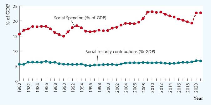
^[1]Joseph Rowntree Foundation, “UK Poverty 2022: The Essential Guide to Understanding Poverty in the UK,” January 18, 2022, https://www.jrf.org.uk/report/uk-poverty-2022.

Support Allowance (ESA), Pension Credit, Housing Benefits, and Working Tax Credit—are all means-tested and meant for people who have limited incomes and capital. Contributory benefits (Social Insurance), which require some eligibility criteria, such as prior contributions to National Insurance, include State Pensions, Employment Support Allowances and Jobseeker's Allowances. Finally, there are noncontributory benefits such as Child Benefits, Disability Living Allowance, Personal Independence Payments, and Carer's Allowances.

Under recent reforms, measures are being implemented to simplify the wel­fare system, reduce wastage, and improve efficiency. For example, Universal Credit is replacing the following benefits: Child Tax Credit, Housing Benefit, Income Support, JSA, ESA, and Working Tax Credits. The contributory JSA/ ESA is also being replaced with a New Style JSA/ESA, which is paid to eligible claimants who are unable to work due to ill health or disability. Paid fortnightly, claimants of this New Style JSA/ESA together with the Universal Credit will have their Universal Credit payment reduced by the New Style ESA amount.

Are sustainability concerns warranted? Current trends and reforms suggest a recognition that the efficiency of the social security system needs to be improved. The system remains deeply woven into the fabric of the United Kingdom's culture and continues to enjoy political support, but ongoing reforms aimed at improving efficiency suggest that, despite its challenges, the system will remain viable.

The Burden of the Government Debt on Future Generations

People often express concern that the trillions of dollars of Federal government debt will impose a crushing financial burden on their children and grandchildren, who will someday be taxed to pay off these debts. In this view, high rates of government borrowing amount to "robbing the future" to pay for government spending that is too high or taxes that are too low in the present. In addition, some researchers have associated high levels of government debt relative to GDP with lower GDP growth.¹⁸

Until recently, it was reasonable to argue that most U.S. government bonds are owned by U.S. citizens. Therefore, although our descendants someday may face heavy taxes to pay the interest and principal of the government debt, these future taxpayers also will inherit outstanding government bonds and thus will be the recipients of most of those interest and principal payments. In that case, one could

¹⁷Social Security Advisory Committee, "SSAC Occasional Paper 26: The Future of Working Age Contributory Benefits for Those Not in Paid Work," GOV.UK, October 24, 2022, (https:llwww.gov.ukl government∕publications∕ssac-occasional-paper-26-the-future-of-working-age-contributory-benefits-for-those-not- in-paid-work).

¹⁸See Carmen M. Reinhart, Vincent R. Reinhart, and Kenneth S. Rogoff, "Debt Overhangs: Past and Present," Journal of Economic Perspectives, Summer 2012, pp. 69-86; and Thomas Herndon, Michael Ash, and Robert Pollin, "Does High Public Debt Consistently Stifle Economic Growth? A Critique of Reinhart and Rogoff," University of Massachusetts Amherst, Political Economy Research Institute working paper, April 2013. argue that to a substantial degree, we owe the government debt to ourselves, so the debt isn't a burden in the same sense that it would be if it were owed entirely to outsiders. However, over the past 25 years, investors, institutions, and govern­ments in other countries—most notably, China—have bought large amounts of U.S. government debt. Since 2001, foreigners have owned more than 30% of all publicly owned U.S. government debt. So, the argument that the debt is not a bur­den because we owe it to ourselves is no longer valid.

Although the popular view of the burden of the government debt is faulty, economists have pointed out several ways in which the government debt can become a burden on future generations. First, if tax rates have to be raised sub­stantially in the future to pay off the debt, the resulting distortions could cause the economy to function less efficiently and impose costs on future generations.

Second, most people hold small amounts of government bonds or no govern­ment bonds at all (except perhaps indirectly, as through pension funds). In the future, people who hold few or no bonds may have to pay more in taxes to pay off the gov­ernment debt than they receive in interest and principal payments; people holding large quantities of bonds may receive more in interest and principal than they pay in increased taxes. Bondholders are richer on average than nonbondholders, so the need to service the government debt might lead to a transfer of resources from the relatively poor to the relatively rich. However, this transfer could be offset by other tax and transfer policies—for example, by raising taxes on high-income people.

The third argument is probably the most significant: Many economists claim that government deficits reduce national saving; that is, when the government runs a deficit, the economy accumulates less domestic capital and fewer foreign assets than it would have if the deficit had been lower. If this argument is correct, deficits will lower the standard of living for our children and grandchildren, both because they will inherit a smaller capital stock and because they will have to pay more interest to (or receive less interest from) foreigners than they otherwise would have. This reduction in the future standard of living would constitute a true burden of the government debt.

Crucial to this argument, however, is the idea that government budget deficits reduce national saving. As we have mentioned at several points in this book (nota­bly in Chapter 4), the question of whether budget deficits affect national saving is highly controversial. We devote most of the rest of this section to further discus­sion of this issue.

Budget Deficits and National Saving: Ricardian Equivalence Revisited

Under what circumstances will an increased government budget deficit cause national saving to fall? Virtually all economists agree that an increase in the deficit caused by a rise in government purchases—say, to fight a war—reduces national saving and imposes a real burden on the economy. However, whether a deficit caused by a cut in current taxes or an increase in current transfers reduces national saving is much less clear. Recall that advocates of Ricardian equivalence argue that tax cuts or increases in transfers will not affect national saving, whereas its opponents disagree.

Ricardian Equivalence: An Example. To illustrate Ricardian equivalence let's suppose that, holding its current and planned future purchases constant, the government cuts this year's taxes by $100 per person. (Assuming that the tax cut is a lump sum allows us to ignore incentive effects.) What impact will this reduc­tion in taxes have on national saving? In answering this question, we first recall the definition of national saving (Eq. 2.8):

S = Y - C - G. (15.5)

Equation (15.5) states that national saving, S, equals output, Y, less consump­tion, C, and government purchases, G.^[292] If we assume that government purchases, G, are constant and that output, Y, is fixed at its full-employment level, we know from Eq. (15.5) that the tax cut will reduce national saving, S, only if it causes con­sumption, C, to rise. Advocates of Ricardian equivalence assert that, if current and planned future government purchases are unchanged, a tax cut will not affect con­sumption and thus won't affect national saving.

Why wouldn't a tax cut that raises after-tax incomes cause people to consume more? The answer is that—if current and planned future government purchases don't change—a tax cut today must be accompanied by an offsetting increase in expected future taxes. To see why, note that if current taxes are reduced by $100 per person without any change in government purchases, the government must bor­row an additional $100 per person by selling bonds. Suppose that the bonds are one-year bonds that pay a real interest rate, r. In the following year, when the gov­ernment repays the principal ($100 per person) and interest ($100 ? r per person) on the bonds, it will have to collect an additional $100(1 + r) per person in taxes. Thus, when the public learns of the current tax cut of $100 per person, they should also expect their taxes to increase by $100( 1 + r) per person next year.^[293]

Because the current tax cut is balanced by an increase in expected future taxes, it doesn't make taxpayers any better off in the long run despite raising their cur­rent after-tax incomes. Indeed, after the tax cut, taxpayers' abilities to consume today and in the future are the same as they were originally. That is, if no one consumes more in response to the tax cut—so that each person saves the entire $100 increase in after-tax income—in the following year the $100 per person of additional saving will grow to $100( 1 + r) per person. This additional $100( 1 + r) per person is precisely the amount needed to pay the extra taxes that will be levied in the future, leaving people able to consume as much in the future as they had originally planned. Because people aren't made better off by the tax cut (which must be cou­pled with a future tax increase), they have no reason to consume more today. Thus national saving should be unaffected by the tax cut, as supporters of Ricardian equivalence claim.

Ricardian Equivalence Across Generations. The argument for Ricardian equivalence rests on the assumption that current government borrowing will be repaid within the lifetimes of people who are alive today. In other words, any tax cuts received today are offset by the higher taxes that people must pay later. But what if some of the debt the government is accumulating will be repaid not by the people who receive the tax cut but by their children or grandchildren? In that case, wouldn't people react to a tax cut by consuming more?

Harvard economist Robert Barro^[294] has shown that, in theory, Ricardian equiv­alence may still apply even if the current generation receives the tax cut and future generations bear the burden of repaying the government's debt. To state Barro's argument in its simplest form, let's imagine an economy in which every genera­tion has the same number of people and suppose that the current generation receives a tax cut of $100 per person. With government purchases held constant, this tax cut increases the government's borrowing and outstanding debt by $100 per person. However, people currently alive are not taxed to repay this debt; instead, this obligation is deferred until the next generation. To repay the govern­ment's increased debt, the next generation's taxes (in real terms) will be raised by $100 (1 + ρ) per person, where 1 + ρ is the real value of a dollar borrowed today at the time the debt is repaid.^[295]

Seemingly, the current generation of people, who receive the tax cut, should increase their consumption because the reduction in their taxes isn't expected to be balanced by an increase in taxes during their lifetimes. However, Barro argued that people in the current generation shouldn't increase their consumption in response to a tax cut if they care about the well-being of the next generation. Of course, people do care about the well-being of their children, as is reflected in part in the economic resources devoted to children, including funds spent on children's health and education, gifts, and inheritances.

How does the concern of this generation for the next affect the response of people to a tax cut? A member of the current generation who receives a tax cut— call him Joel—might be inclined to increase his own consumption, all else being equal. But, Barro argues, Joel should realize that, for each dollar of tax cut he receives today, his child Joel Junior will have to pay 1 + ρ dollars of extra taxes in the future. Can Joel do anything on his own to help out Joel Junior? The answer is yes. Suppose that, instead of consuming his $100 tax cut, Joel saves the $100 and uses the extra savings to increase Joel Junior's inheritance. By the time the next generation is required to pay the government debt, Joel Junior 's extra inheritance plus accumulated interest will be $100( 1 + ρ), or just enough to cover the increase in Joel Junior 's taxes. Thus by saving his tax cut and adding these savings to his planned bequest, Joel can keep both his own consumption and Joel Junior's con­sumption the same as they would have been if the tax cut had never occurred.

Furthermore, Barro points out, Joel should save all his tax cut for Joel Junior's benefit. Why? If Joel consumes even part of his tax cut, he won't leave enough extra inheritance to allow Joel Junior to pay the expected increase in his taxes, and so Joel Junior will have to consume less than he could have if there had been no tax cut for Joel. But if Joel wanted to increase his own consumption at Joel Junior's expense, he could have done so without changes in the tax laws—for example, by contributing less to Joel Junior 's college tuition payments or by planning to leave a smaller inher­itance. That Joel didn't take these actions shows that he was satisfied with the divi­sion of consumption between himself and Joel Junior that he had planned before the tax cut was enacted; there is no reason that the tax cut should cause this original consumption plan to change. Therefore if Joel and other members of the current generation don't consume more in response to a tax cut, Ricardian equivalence should hold even when debt repayment is deferred to the next generation.

This analysis can be extended to allow for multiple generations and in other ways. These extensions don't change the main point, which is that, if taxpayers understand that they are ultimately responsible for the government's debt, they shouldn't change their consumption in response to changes in taxes or transfers that are unaccompanied by changes in planned government purchases. As a result, deficits created by tax cuts shouldn't reduce national saving and therefore shouldn't burden future generations.

Departures from Ricardian Equivalence

The arguments for Ricardian equivalence are logically sound, and this idea has greatly influenced economists' thinking about deficits. Although 40 years ago most economists would have taken for granted that a tax cut would substantially increase consumption, today there is much less agreement about this claim. Although Ricardian equivalence seemed to fail spectacularly in the 1980s in the United States—when high government budget deficits were accompanied by extremely low rates of national saving—data covering longer periods of time sug­gest little relationship between budget deficits and national saving rates in the United States. In some other countries, such as Canada and Israel, Ricardian equivalence seems to have worked quite well at times.^[296]

Our judgment is that tax cuts that lead to increased government borrowing probably affect consumption and national saving, although the effect may be small. We base this conclusion both on the experience of the United States during the 1980s and on the fact that there are some theoretical reasons to expect Ricardian equiva­lence not to hold exactly. The main arguments against Ricardian equivalence are the possible existence of borrowing constraints, consumers' shortsightedness, the failure of some people to leave bequests, and the non-lump-sum nature of most tax changes.

1. Borrowing constraints. Many people would be willing to consume more if they could find lenders who would extend them credit. However, consumers often face limits, known as borrowing constraints, on the amounts that they can borrow. A person who wants to consume more, but who is unable to borrow to do so, will be eager to take advantage of a tax cut to increase consumption. Thus the existence of borrowing constraints may cause Ricardian equivalence to fail.

2. Shortsightedness. In the view of some economists, many people are short­sighted and don't understand that as taxpayers they are ultimately responsi­ble for the government's debt. For example, some people may determine their consumption by simple "rules of thumb," such as the rule that a family should spend fixed percentages of its current after-tax income on food, clothing, housing, and so on, without regard for how its income is likely to change in the future. If people are shortsighted, they may respond to a tax cut by con­suming more, contrary to the prediction of Ricardian equivalence. However, Ricardians could reply that ultrasophisticated analyses of fiscal policy by con­sumers aren't necessary for Ricardian equivalence to be approximately cor­rect. For example, if people know generally that big government deficits mean future problems for the economy (without knowing exactly why), they may be reluctant to spend from a tax cut that causes the deficit to balloon, consis­tent with the Ricardian prediction.

3. Failure to leave bequests. If people don't leave bequests, perhaps because they don't care or think about the long-run economic welfare of their children, they will increase their consumption if their taxes are cut, and Ricardian equiva­lence won't hold. Some people may not leave bequests because they expect their children to be richer than they are and thus not need any bequest. If people continue to hold this belief after they receive a tax cut, they will increase their consumption and again Ricardian equivalence will fail.

4. Non-lump-sum taxes. In theory, Ricardian equivalence holds only for lump­sum tax changes, with each person's change in taxes being a fixed amount that doesn't depend on the person's economic decisions, such as how much to work or save. As discussed in Section 15.2, when taxes are not lump-sum, the level and timing of taxes will affect incentives and thus economic behavior. Thus non-lump-sum tax cuts will have real effects on the economy, in contrast to the simple Ricardian view.

We emphasize, though, that with non-lump-sum taxes, the incentive effects of a tax cut on consumption and saving behavior will depend heavily on the tax structure and on which taxes are cut. For example, a temporary cut in sales taxes would likely stimulate consumption, but a reduction in the tax rate on interest earned on savings accounts might increase saving. Thus we cannot always con­clude that, just because taxes aren't lump-sum, a tax cut will increase consump­tion. That conclusion has to rest primarily on the other three arguments against Ricardian equivalence that we presented.

In Touch with Data and Research

Measuring the Impact of Government Purchases on the Economy

The United Kingdom's Coronavirus Job Retention Scheme, in effect between March 1, 2020, and September 30, 2021, provided grants to employers so they could retain and continue to pay staff during coronavirus-related lockdowns by furloughing employees at up to 80% of their wages. Official government sources reported that 11.7 million jobs were furloughed at a cost of £70 billion, part of an estimated £122 billion put into a form of reverse taxation by HM Revenue and Customs and involving the Self-employed Income Support Scheme. The 2020­2021 fiscal year's government spending reached £1.096 trillion—the first time £1 trillion has ever been surpassed—with a one-year increase of 23.5%.

Although few would argue against the Scheme's usefulness, economists with classical and Keynesian leanings have been debating the effects of the gov­ernment's purchases on aggregate economic activity, with no clear consensus emerging. As consumer spending typically accounts for over 60% of the United Kingdom's aggregate demand, its response is an important determinant of the fis­cal multiplier's size. The standard real business cycle (RBC) and the IS-LM mod­els offer different qualitative predictions. While the IS-LM model predicts that consumption should rise, thereby amplifying the effects of increased government spending on output, the RBC model generally predicts a decline in consumption in response. The different impacts of the two models derive from assumptions about how consumers behave in each case. The RBC model assumes Ricardian households, whose consumption decisions at any point in time are based on an across-time budget constraint; in other words, Ricardian equivalence holds. In the IS-LM model, however, consumers behave in a non-Ricardian fashion, with consumption being a function of current disposable income and not of their life­time resources. To illustrate this using the IS-LM model, a temporary increase in government purchases shifts the IS curve up (and right) (as discussed in Section 9.2, "The IS Curve: Equilibrium in the Goods Market") resulting in a new IS-LM intersection to the right of the former. When prices remain fixed in the short run, as in the Keynesian version of the model, the new intersection implies a short-run output increase.

However, when prices are assumed to adjust quickly, the LM curve shifts up (and left), thereby offsetting the rightward IS curve shift. It is also worth noting that, as discussed in Section 10.2 ("Fiscal Policy Shocks in the Classical Model"), an increase in government spending may be the equivalent of a rise in workers' current or future taxes, with the result that they see themselves as poorer and hence supply more labor, thereby increasing output. In effect, both classical and Keynesian approaches can be used to explain how temporary in­creases in government spending can lead to higher output, albeit through differ­ent mechanisms.

The fiscal multiplier is estimated by determining the short-run national output changes due to a unit change in government spending. However, researchers have noted the difficulty in assigning causality to specific government spending because of other potential shocks that also affect the economy. Further, the choice of the appropriate variable is important. Research by Riera-Crichton, Vegh, and Vuletin (2012) underscores this need. Their analysis, using a novel value-added tax rate dataset and the corresponding cyclically adjusted revenue measured at a quarterly frequency for 14 industrialized countries between 1980 and 2009, strongly sup­ports using tax rates as the true measure of a tax policy.^[297] Further, some studies have found that fiscal multipliers could be different during recessions compared to booms, as there would be less crowding when supply constraints are not binding. Auerbach and Gorodnichenko (2012), for example, found that spending multipliers are significantly higher during recessions.^[298] As discussed in Section 14.2 ("Monetary Control in the United States"), the size of the fiscal multiplier can be impacted by the monetary policy response. Research by Boubaker and colleagues (2018) found that, for the big four eurozone economies (France, Germany, Italy, and Spain), the gov­ernment spending multiplier is above 1.8 when associated with a long-term com­mitment to keeping the nominal interest rate at the zero lower bound.^[299]

As for the United Kingdom, the Office of Budget Responsibility's Economic and Fiscal Outlook reported fiscal multipliers ranging from 0.15 to 1.00 across sev­eral fiscal policy activities for 2020-21.^[300] Overall, evidence from the extant litera­ture indicates that care needs to be taken in estimating fiscal multipliers.

15.4