Government Spending, Taxes, and the Macroeconomy
Describe how government spending and taxing decisions affect the macroeconomy.
How does fiscal policy affect the performance of the macroeconomy? Economists emphasize three main ways by which government spending and taxing decisions influence macroeconomic variables such as output, employment, and prices: (1) aggregate demand, (2) government capital formation, and (3) incentives.
Fiscal Policy and Aggregate Demand
Fiscal policy can affect economic activity by influencing the total amount of spending in the economy, or aggregate demand. Recall that aggregate demand is represented by the intersection of the IS and LM curves. In either the classical or the Keynesian IS-LM model, a temporary increase in government purchases reduces desired national saving and shifts the IS curve up and to the right, thereby raising aggregate demand.
Classical and Keynesian economists have different beliefs about the effect of tax changes on aggregate demand. Classicals usually accept the Ricardian equivalence proposition, which says that lump-sum tax changes do not affect desired national saving and thus have no impact on the IS curve or aggregate demand.4 Keynesians
4We introduced Ricardian equivalence in Chapter 4. We discuss this idea further in Section 15.3. generally disagree with this conclusion; in the Keynesian view, a cut (for example) in taxes is likely to stimulate desired consumption and reduce desired national saving, thereby shifting the IS curve up and to the right and raising aggregate demand.
Classicals and Keynesians also disagree over the question of whether fiscal policy should be used to fight the business cycle. Classicals generally reject attempts to smooth business cycles, by fiscal policy or by other means. In contrast, Keynesians argue that using fiscal policy to stabilize the economy and maintain full employment—for example, by cutting taxes and raising spending when the economy is in a recession—is desirable.
However, even Keynesians admit that the use of fiscal policy as a stabilization tool is difficult. A significant problem is lack of flexibility. The government's budget has many purposes besides macroeconomic stabilization, such as maintaining national security, providing income support for eligible groups, developing the nation's infrastructure (roads, bridges, and public buildings), and supplying government services (education and public health). Much of government spending is committed years in advance (as in weapons development programs) or even decades in advance (as for Social Security benefits). Expanding or contracting total government spending rapidly for macroeconomic stabilization purposes thus is difficult without either spending wastefully or compromising other fiscal policy goals. For instance, when the American Recovery and Reinvestment Act (ARRA) was enacted in 2009 to stimulate the economy, much attention was paid to finding "shovel-ready" projects, that is, projects that could be undertaken immediately. Taxes are somewhat easier to change than spending, but the tax laws also have many different goals and may be the result of a fragile political compromise that isn't easily altered.
Compounding the problem of inflexibility is the problem of long time lags that result from the slow-moving political process by which fiscal policy is made. From the time a spending or tax proposal is made until it goes into effect is rarely less than 18 months. This lag makes effective countercyclical use of fiscal policy difficult because (for example), by the time an antirecession fiscal measure actually had an impact on the economy, the recession might already be over.
Automatic Stabilizers and the Full-Employment Deficit. One way to get around the problems of fiscal policy inflexibility and long lags that impede the use of countercyclical fiscal policies is to build automatic stabilizers into the budget. Automatic stabilizers are provisions in the budget that cause government spending to rise or taxes to fall automatically—without legislative action—when GDP falls.
Similarly, when GDP rises, automatic stabilizers cause spending to fall or taxes to rise without any need for direct legislative action.A good example of an automatic stabilizer is unemployment insurance. When the economy goes into a recession and unemployment rises, more people receive unemployment benefits, which are paid automatically without further action by Congress. Thus the unemployment insurance component of transfers rises during recessions, making fiscal policy automatically more expansionary.[282]
Quantitatively, the most important automatic stabilizer is the income tax system. When the economy goes into a recession, people's incomes fall, and they pay less income tax. This "automatic tax cut" helps cushion the drop in disposable income and (according to Keynesians) prevents aggregate demand from falling as far as it might otherwise. Likewise, when people's incomes rise during a boom,
FIGURE 15.5
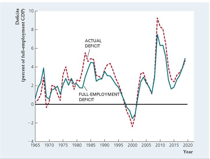
Full-employment and actual budget deficits, 1965-2019
The actual and fullemployment Federal budget deficits are shown as percentages of full-employment output. The actual budget deficit exceeded the fullemployment deficit by substantial amounts during or slightly after the 1973-1975, 1981-1982, 1990-1991, 2001, and 2007-2009 recessions, reflecting the importance of automatic stabilizers. Data are not shown for the pandemic period of 2020-2021 because the CBO did not estimate the full-employment deficit during the pandemic. Source: Congressional Budget Office, www.cbo.gov/system/ files?file=2020-02/51139-2020-02- Uutomaticstabilizers.xlsx.
the government collects more income tax revenue, which helps restrain the increase in aggregate demand. Keynesians argue that this automatic fiscal policy is a major reason for the increased stability of the economy since World War II.
A side effect of automatic stabilizers is that government budget deficits tend to increase in recessions because government spending automatically rises and taxes automatically fall when GDP declines.
Similarly, the deficit tends to fall in booms. To distinguish changes in the deficit caused by recessions or booms from changes caused by other factors, some economists advocate the use of a deficit measure called the fullemployment deficit. The full-employment deficit indicates what the government budget deficit would be—given the tax and spending policies currently in force—if the economy were operating at its full-employment level.[283] Because it eliminates the effects of automatic stabilizers, the full-employment deficit measure is affected primarily by changes in fiscal policy reflected in new legislation. In particular, expansionary fiscal changes—such as increases in government spending programs or (in the Keynesian model) reduced tax rates—raise the full-employment budget deficit, whereas contractionary fiscal changes reduce the full-employment deficit.Figure 15.5 shows the actual and full-employment budget deficits (as percentages of full-employment output) of the Federal government since 1965. Note that the actual budget deficit substantially exceeded the full-employment budget deficit during or slightly after the recessions of 1973-1975, 1981-1982, 1990-1991, 2001, and 2007-2009 when output was below its full-employment level. The difference between the two deficit measures reflects the importance of automatic stabilizers in the budget.
Government Capital Formation
The health of the economy depends not only on how much the government spends but also on how it spends its resources. For example, as discussed in Chapter 6, the quantity and quality of public infrastructure—roads, schools, public hospitals, and the like—are potentially important for the rate of economic growth. Thus the formation of government capital—long-lived physical assets owned by the government— is one way that fiscal policy affects the macroeconomy. The government budget affects not only physical capital formation but also human capital formation.
At least part of government expenditures on health, nutrition, and education are an investment, in the sense that they will lead to a more productive work force in the future.The official figures for government capital investment focus on physical capital formation and exclude human capital formation. In 2021 Federal government investment expenditures were $360 billion (about 23% of Federal purchases of goods and services), with 55% of investment spending for national defense and 45% for nondefense government capital. State and local government investment was $442.3 billion (about one-sixth of state and local government purchases of goods and services). The composition of government investment by state and local governments differs from that by the Federal government. Most Federal government investment is in the form of intellectual property products (such as research and development) rather than equipment or structures, but about three- quarters of state and local government investment is for structures.
Incentive Effects of Fiscal Policy
The third way in which fiscal policy affects the macroeconomy is by its effects on incentives. Tax policies in particular can affect economic behavior by changing the financial rewards to various activities. For example, in Chapter 4 we showed how tax rates influence the incentives of households to save and of firms to make capital investments.
Average Versus Marginal Tax Rates. To analyze the effects of taxes on economic incentives, we need to distinguish between average and marginal tax rates. The average tax rate is the total amount of taxes paid by a person (or a firm), divided by the person's before-tax income. The marginal tax rate is the fraction of an additional dollar of income that must be paid in taxes. For example, suppose that in a particular country no taxes are levied on the first $10,000 of income and that a 25% tax is levied on all income above $10,000 (see Table 15.3). Under this income tax system a person with an income of $18,000 pays a tax of $2000.
Thus her average tax rate is 11.1% ($2000 in taxes divided by $18,000 in before-tax income). However, this taxpayer's marginal tax rate is 25% because a $1.00 increase in her income will increase her taxes by $0.25. Table 15.3 shows that everyone with an income higher than $10,000 faces the same marginal tax rate of 25% but that the average tax rate increases with income.We can show why the distinction between average and marginal tax rates is important by considering the individual's decision about how much labor to supply. The effects of a tax increase on the amount of labor supplied depend strongly on whether average or marginal taxes are being increased. Economic theory predicts that an increase in the average tax rate, with the marginal tax rate held constant, will increase the amount of labor supplied at any (before-tax) real wage. In contrast,
TABLE 15.3
| Marginal and Average Tax Rates: An Example (Total Tax = 25% of Income More Than $10,000) | ||||
| Income | Income-$10,000 | Tax | Average tax rate | Marginal tax rate |
| $ 18,000 | $ 8,000 | $ 2,000 | 11.1% | 25% |
| 50,000 | 40,000 | 10,000 | 20.0% | 25% |
| 100,000 | 90,000 | 22,500 | 22.5% | 25% |
the theory predicts that an increase in the marginal tax rate, with the average tax rate held constant, will decrease the amount of labor supplied at any real wage.
To explain these conclusions, let's first consider the effects of a change in the average tax rate. Returning to our example from Table 15.3, imagine that the marginal tax rate stays at 25% but that now all income over $8000 (rather than all income more than $10,000) is subject to a 25% tax. The taxpayer with an income of $18,000 finds that her tax bill has risen from $2000 to $2500, or 0.25 ($18,000 — $8000), so her average tax rate has risen from 11.1% to 13.9%, or $2500/$18,000. As a result, the taxpayer is $500 poorer. Because she is effectively less wealthy, she will increase the amount of labor she supplies at any real wage (see Summary table 4 in Chapter 3). Hence an increase in the average tax rate, holding the marginal tax rate fixed, shifts the labor supply curve (in a diagram with the before-tax real wage on the vertical axis) to the right.[284]
Now consider the effects of an increase in the marginal tax rate, with the average tax rate constant. Suppose that the marginal tax rate on income increases from 25% to 40% and the rise is accompanied by other changes in the tax law that keep the average tax rate—and thus the total amount of taxes paid by the typical taxpayer—the same. To be specific, suppose that the portion of income not subject to tax is increased from $10,000 to $13,000. Then for the taxpayer earning $18,000, total taxes are $2000, or 0.40( $18,000 — $13,000), and the average tax rate of 11.1%, or $2000/$18,000, is the same as it was under the original tax law.[285]
With the average tax rate unchanged, the taxpayer 's wealth is unaffected, and so there is no change in labor supply stemming from a change in wealth. However, the increase in the marginal tax rate implies that the taxpayer 's after-tax reward for each extra hour worked declines. For example, if her wage is $20 per hour before taxes, at the original marginal tax rate of 25%, her actual take-home pay for each extra hour of work is $15 ($20 minus 25% of $20, or $5, in taxes). At the new marginal tax rate of 40%, the taxpayer 's take-home pay for each extra hour of work is only $12 ($20 in before-tax wages minus $8 in taxes). Because extra hours of work no longer carry as much reward in terms of real income earned, at any specific before-tax real wage the taxpayer is likely to work fewer hours and enjoy more leisure instead. Thus, if the average tax rate is held fixed, an increase in the marginal tax rate causes the labor supply curve to shift to the left.[286]
The Tax Act of 2017 reduced marginal tax rates for most taxpayers in 2018, but these reductions were legislated to be temporary. The decline in marginal tax rates was designed to encourage economic activity, and our theory says this should cause labor supply curves to shift to the right. Econometric estimates of the effect suggested that the decline in the marginal tax rates might have increased GDP growth by about 0.9 percentage points in 2019 but not much after that.[287] The tax changes in 2017 also reduced business taxation, which might have a longer-lasting impact on output through increased incentives for investment, leading to a higher capital stock. However, measuring the actual impact of these tax changes was difficult because of the pandemic's effects in 2020 and 2021.
Tax-Induced Distortions and Tax Rate Smoothing. Because taxes affect economic incentives, they change the pattern of economic behavior. If the invisible hand of free markets is working properly, the pattern of economic activity in the absence of taxes is the most efficient, so changes in behavior caused by taxes reduce economic welfare. Tax-induced deviations from efficient, free-market outcomes are called distortions.
To illustrate the idea of a distortion, let's go back to the example of the worker whose before-tax real wage is $20. Because profit-maximizing employers demand labor up to the point that the marginal product of labor equals the real wage, the real output produced by an extra hour of the worker's labor (her marginal product) also is $20. Now suppose that the worker is willing to sacrifice leisure to work an extra hour if she receives at least $14 in additional real earnings. Because the value of what the worker can produce in an extra hour of labor exceeds the value that she places on an extra hour of leisure, her working the extra hour is economically efficient.
In an economy without taxes, this efficient outcome occurs because the worker is willing to work the extra hour for the extra $20 in real wages. She would also be willing to work the extra hour if the marginal tax rate on earnings was 25% because at a marginal tax rate of 25% her after-tax real wage is $15, which exceeds the $14 real wage minimum that she is willing to accept. However, if the marginal tax rate rises to 40%, so that the worker's after-tax wage falls to only $12, she would decide that it isn't worth her while to work the extra hour, even though for her to do so would have been economically efficient. The difference between the number of hours the worker would have worked had there been no tax on wages and the number of hours she actually works when there is a tax reflects the distorting effect of the tax. The higher the tax rate is, the greater the distortion is likely to be.
Because doing without taxes entirely isn't possible, the problem for fiscal policymakers is how to raise needed government revenues while keeping distortions relatively small. Because high tax rates are particularly costly in terms of economic efficiency, economists argue that keeping tax rates roughly constant at a moderate level is preferable to alternate periods of very low and very high tax rates. For example, if the government's spending plans require it to levy a tax rate that over a number of years averages 20%, most economists would advise the government not to set the tax rate at 30% half the time and 10% the other half. The reason is the large distortions that the 30% tax rate would cause in the years that it was effective. A better strategy is to hold the tax rate constant at 20%. A policy of maintaining stable tax rates so as to minimize distortions is called tax rate smoothing.
Application
Supply-Side Economics
Economic incentives play a significant role in influencing economic agents' decisions. Intuitively, the higher the benefits associated with an activity, the higher the incentive. Although economic output is the outcome of the interaction of aggregate supply (AS) and aggregate demand (AD), supply-side economics focuses on AS and is based on the idea that efficient supply of goods and services within the economy is a main driver of long-term growth. Broadly, it is concerned with the determinants of potential output, or productive capacity, and changes. Originating in the United States in the mid-1970s, the term gained prominence in the 1980s under UK prime minister Margaret Thatcher and U.S. president Ronald Reagan. As an intertemporal approach, supply-side economics focuses on the effects of today's actions over time and on the effects of expected action on today's behavior.
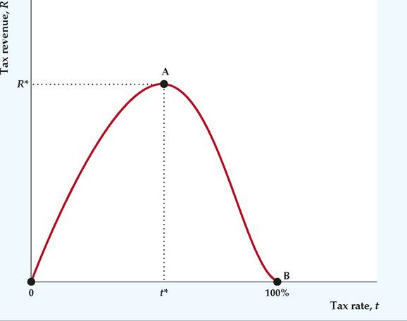
One of the main means of incentivizing economic agents to increase supply is through tax policy, and "supply-siders" argue that labor supply, productivity, savings, and investments respond positively to tax incentives through their significant effect on these variables. Supply-side economics is often visually represented by the so-called Laffer curve, which charts the theoretical relationship between tax rates and tax revenue. The curve, created by the U.S. economist Arthur Laffer, argues that beyond a certain tax level, lowering tax rates improves tax revenue through higher economic growth. The basis is that at a constant tax-rate of t and labor income Y, tax revenue (R = tY) is increased when t is reduced as it incentivizes a bigger increase in Y. The Laffer curve (Figure 15.6) is motivated by three intuitive observations. First, when t = 0%, R = 0, (shown at point O). Second, when t = 100%, there will be no incentive to work (discounting totally altruistic considerations) and labor income will be zero; therefore, R = 0 (shown at point B). Third, for 0% < t < 100%, workers will supply labor, earn incomes, and pay income taxes, resulting in positive tax revenue (R > 0). Since R = 0 for t = 0% and t = 100% and tax revenue is positive for 0% < t < 100%, the Laffer curve will have to peak at some point, t*, which provides government with the highest tax revenue, R*. In countries where supply-siders push for marginal tax-rate reductions, their argument is that t is on the right-side of t*, so reductions in t will increase R. Put differently, below t*, the marginal tax revenue raised decreases as t increases, until it reaches t* (point A, where the slope of the Laffer curve becomes zero). Beyond t*, any tax-rate increases reduce tax revenue.
Based on the above explanation, the importance of getting t* right cannot be overstated. However, most of the empirical evidence advanced to support the supply-siders' position concerns U.S. economic policy. An obvious problem with any empirical test of the Laffer curve's effects in most countries is the paucity of data available.
To test the Laffer curve's relevance on a broader scale, the Fiscal Affairs Department of the IMF conducted a project in 1984 analyzing the relevance to developing countries of the tax policy recommendations of supply-side economics made in the context of developed countries. The results were, at best, mixed. Ebrill, analyzing 1970s data for Jamaica and India, concludes that, although there is some evidence of tax revenue buoyancy in Jamaica, the opposite was found
(continued)
FIGURE 15.6
The Laffer curve
At tax rates of 0% and 100%, the government collects no tax revenue. Beginning with a tax rate of 0%, increasing the tax rate leads to increased tax revenue. But as the tax rate continues to rise, tax revenue grows less and less as people work less. For tax rates above t*, a higher tax rate leads to lower tax revenues.
in India.11 For India, the "revenue performance" of the highest income group was rather poor even though this group, which included taxpayers that had the greatest marginal tax-rate reduction (20.75 percentage points), should have exhibited the most pronounced Laffer-type effects. Analyzing Korean data, Ohchul Kwon, an American economist, concluded that the behavior of tax revenues over time as tax rates were increased was not inconsistent with the existence of a Laffer curve.[288] [289] Kwon showed that when the marginal tax rate increased from 4.3% in 1972 to 17.8% in 1974, tax revenue rose at increasing rates from 6.3% to 56.3%. However, as the marginal tax rate increased from 17.8% in 1974 to 22.3% in 1976, tax revenue increased at decreased rates from 56.3% to 49.5%.
Proponents argue that supply-side policies can help reduce inflationary pressures in the long term because of efficiency and productivity gains in the product and labor markets; it can also help create real jobs and sustainable growth through their positive effect on labor productivity and competitiveness. However, such policies must be implemented cautiously. In 2022, shortly after taking office, former UK prime minister Liz Truss rashly implemented a broad set of supply-side fiscal policies, including significant tax cuts and spending plans. However, markets reacted unfavorably, leading to a sudden and sharp devaluation of the British pound to historically low levels, accompanied by mounting inflation. Critics argue that relying on supply alone does not create demand. Moreover, it can take a long time to work its way through the economy. Yet supply-side economics remains an important policymaking tool, even as identifying the optimal tax-rate remains a non-trivial task, as does knowing which income groups should get tax reductions to increase tax revenues.
Has the Federal government had a policy of tax rate smoothing? Statistical studies typically have found that Federal tax rates are affected by political and other factors and hence aren't as smooth as is necessary to minimize distortions.13 Nevertheless, the idea of tax smoothing is still useful. For example, what explains the U.S. government's huge deficit during World War II (Fig. 15.4)? The alternative to deficit financing of the war would have been a large wartime increase in tax rates, coupled with a drop in tax rates when the war was over. But high tax rates during the war would have distorted the economy when productive efficiency was especially important. By financing the war largely through borrowing, the government effectively spread the needed tax increase over a long period of time (as the debt was repaid) rather than raising current taxes by a large amount. This action is consistent with the idea of tax smoothing.
15.2
More on the topic Government Spending, Taxes, and the Macroeconomy:
- CONCLUSIONS: MAJOR FINDINGS FROM THE LITERATURE SURVEY AND IMPLICATIONS FOR FURTHER RESEARCH
- Portugal
- Index