Growth with Expanding Product Varieties
Finally, we will briefly discuss the equivalent model in which growth is driven by product innovations, that is, by expanding product varieties rather than expanding varieties of inputs.
The economy is in continuous time and has constant population L. It admits a representative household with preferences given by
where
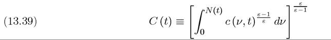
is the consumption index, which is a CES aggregate of the consumption of different varieties. Here c (ν, t) denotes the consumption of product ν at time t, while N (t) is the total measure of products. We assume throughout that ε > 1. Therefore, we have replaced expanding input varieties with expanding product varieties. The log specification in this utility function is for simplicity, and can be replaced by a CRRA utility function.
The patent to produce each product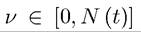 belongs to a monopolist, and the
monopolist who invents the blueprints for a new product receives a fully enforced perpetual 491
patent on this product. Each product can be produced with the technology
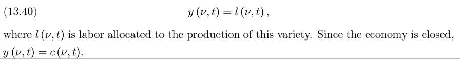
As in model with knowledge spillovers of Section 13.2, we assume that new products can be produced with the production function

The reader will notice that there is a very close connection between the model here and the models of expanding input variety studied so far, especially the model with knowledge spillovers in Section 13.2. For instance, if y (ν, t)s were interpreted as intermediate goods or inputs instead of products and if C (t) in (13.39) were interpreted as the production function for the final good rather than part of the utility function of the representative consumer, the two models would be essentially identical.
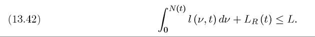
The only difference would be that, with this interpretation, labor would now be used in the production of the inputs, while in Section 13.2 it is used in the final good sector. This similarity emphasizes that the distinction between process and product innovations is fairly minor in theory, though this distinction might still be useful in mapping these models to reality.An equilibrium and a balanced growth path are defined similarly to before. The representative household now determines both the allocation of its expenditure on different varieties and the time path of consumption expenditures. We assume that the economy is closed and there is no capital, thus all output must be consumed. Nevertheless, the consumer Euler equation will apply to determine the equilibrium interest rate. Labor market clearing requires that
Let us start with expenditure decisions. Since the representative household has Dixit- Stiglitz preferences, the following consumer demands can be derived (see Exercise 13.24): 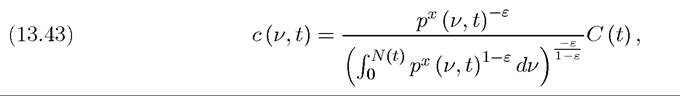 where px (ν, t) is the price of product variety ν at time t, and C (t) is defined in (13.39). The term in the denominator is the ideal price index raised to the power —ε. As before, it is most convenience to set this ideal price index as the numeraire, so that the price of output at every instant is normalized to 1. Thus we impose
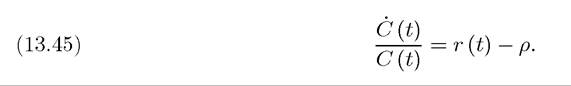
With this choice of numeraire, we obtain the consumer Euler equation as (see Exercise 13.25):
With similar arguments to before, the net present discounted value of the monopolist owning the patent for product ν can be written as

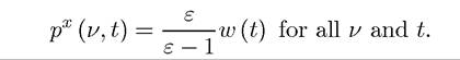
where w (t) c(ν, t) is the total expenditure of the firm to produce a total quantity of c(ν, t) (given the production function (13.40) and the wage rate at time t equal to w (t)), while 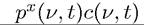 is its revenue, consistent with the demand function (13.43).
Since all firms charge the same price, they will all produce the same amount and employ the same amount of labor. At time t, there are N (t) products, so the labor market clearing condition (13.42) implies that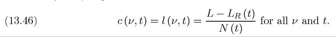
Consequently, the instantaneous profits of each monopolist at time t can be written as
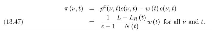
Since prices, sales and profits are equal for all monopolists, we can simplify notation by letting
In addition, since c(ν, t) = c (t) for all ν,
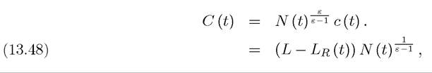
where the second equality uses (13.46).
Labor demand comes from the research sector as well as from the final good producers. Labor demand from research can again be determined using the free entry condition. Assuming that there is positive research, so that the free entry condition holds as an equality, this takes the form
Combining this equation with (13.47), we see that  where we use π (t) to denote the profits of all monopolists at time t, which are equal. In BGP, where the fraction of the workforce working in research is constant, this implies that profits and the net present discounted value of monopolists are also constant. Moreover, in this case we must have
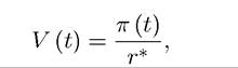
where r* denotes the BGP interest rate.
The previous two equations then imply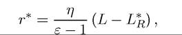
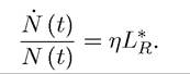
with. denoting the BGP size of the research sector. The R&D employment level of
 combined with the R&D sector production function, (13.41) then implies
However, we also know from the consumer Euler equation, (13.45) combined with (13.48) 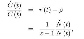 which implies
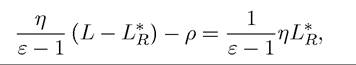
or
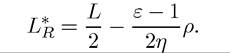
Consequently, the growth rate of consumption expenditure (and utility) is
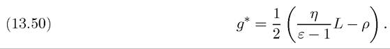
This establishes:
Proposition 13.6. In the above-described expanding product variety model, there exists a unique BGP, in which aggregate consumption expenditure, C (t), grows at the rate g* given by (13.50).
A couple of features are worth noting about this equilibrium. First, in this equilibrium, there is growth of “real income,” even though the production function of each good remains unchanged. This is because, while there is no process innovation reducing costs or improving quality, the number of products available to consumers expands because of product innovations. Since the utility function of the representative household, (13.38), exhibits love-for-variety, the expanding variety of products increases utility. What happens to income 494
depends on what we choose as the numeraire. The natural numeraire is the one setting the ideal price index, (13.44), equal to 1, which amounts to measuring incomes in similar units at different dates.
With this choice of numeraire, real incomes grow at the same rate as C (t), at the rate g*. Second, even though the equilibrium was characterized in a somewhat different manner than our baseline expanding input variety model, there is a close parallel between expanding product varieties and expanding input varieties. This can be seen, for example, in Exercise 13.23, which looks at an economy with expanding input varieties produced by labor. It can be verified that the structure of the equilibrium is very similar to the one studied here. Third, Exercise 13.26 will show that as in the other models of endogenous technological progress we have seen in this chapter, there are no transitional dynamics and the equilibrium is again Pareto suboptimal. Moreover, log preferences now ensure that the transversality condition is always satisfied. Finally, it can be verified that there is again a scale effect here. This discussion then reveals that whether one wishes to use the expanding input variety or the expanding product model is mostly a matter of taste, and perhaps one of context. Both models lead to a similar structure of equilibria, to similar equilibrium growth rates, and to similar welfare properties.13.3.
More on the topic Growth with Expanding Product Varieties:
- Growth with Expanding Product Varieties
- The previous chapter presented the basic endogenous technological change models based on expanding input or product varieties.
- The previous chapter presented the basic endogenous technological change models based on expanding input or product varieties.
- References and Literature
- Baseline Model of Directed Technological Change
- The Lab Equipment Model of Growth with Input Varieties
- References and Literature
- Taking Stock
- Acemoglu Daron. Introduction to Modern Economic Growth: Parts 1-4. Department of Economics, Massachusetts Institute of Technology,2008. — 604 p., 2008
- Acemoglu D.. Introduction to Modern Economic Growth. Princeton University Press,2008. — 1248 p., 2008