Imperfect Information and the Nonneutrality of Money

The short-run neutrality of money implied by new classical models was troublesome for some of their proponents, as these models were not compatible with the evidence suggesting the existence of a positive short-run relation between inflation and employment.⁶

Lucas [1972] responded by developing a new classical model that was consistent with a positive short-run relation between inflation and employment, even under rational expectations.

This model was later extended by Alogoskoufis [1983] to explicitly incorporate competitive labor markets. The assumption in this extended model is that households make their labor supply decisions in the absence of full information about the price level. They are assumed to only observe their nominal wage and the price of the product of the firm for which they work. Hence, when they observe their wage and the price of their firm’s output rise unexpectedly, they systematically attribute this rise to a change in the relative price of their output and their real wage. Thus, employment and output rise in response to unanticipated inflation, as labor supply rises in response to the increased labor demand by firms.

It is this extended version of the Lucas [1972] model that we shall examine, as this model incorporates the labor market and is thus compatible with the perfectly competitive model presented in section 14.1.

14.3.1 Competitive Equilibrium under Imperfect Information about the Price Level

Assume a competitive economy that is described by the new classical model of section 14.1. However, following Lucas [1972], let us assume that current production takes place in a continuum of “islands,” which are informationally isolated.

Production takes place at the beginning of each period, with producers having only local information about prices and wages. Consumption is decided at the end of each period, under full information about prices and interest rates, and all consumers consume a composite commodity consisting of the products of all islands. Islands are indexed by z, where z ∈ [0, 1].

Under these assumptions, employment, output, nominal wages, and prices are determined at the local level, with firms and producers having no information about current wages and prices on the other islands when they make their production and labor supply decisions. Employment, output, nominal wages, and nominal prices on island z are determined under imperfect information, by the equality of labor supply with labor demand, and output supply with output demand on island z. They are thus determined by

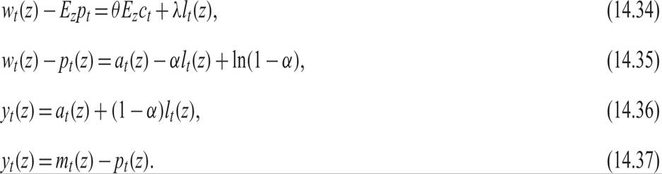
All variables in these equations are in logarithms. Here w(z) is the nominal wage in island z; p(z) is the competitive price of the good produced in island z; l(z) is employment in island z, determined by the equality of labor demand with labor supply; y(z) is output in island z, determined by the equality of supply and demand; E_zp_t denotes the rational expectation about the end-period price level, based on the local information set for island z at the beginning of period t; E_zc_t denotes the rational expectation about the end-period household consumption, conditional on local information at the beginning of the period; a(z) is labor productivity in island z, and m(z) is the money supply in island z.

Equation (14.34) is the labor supply function of the representative household on island z, derived from the first-order conditions for the maximization of its intertemporal utility derived in the same way as (14.10). Equation (14.35) is the labor demand function of the representative firm on island z derived in the same way as (14.16), by a marginal productivity condition. Equation (14.36) is the log-linearized production function of the representative firm on island z, derived in the same way as (14.17). Equation (14.37) is the demand function for the product of the representative firm on island z. This function depends on the money supply allocated to island z by traders in goods, who collect goods from the various islands at the beginning of the period and sell them to consumers as consumption bundles at the end of the period. The marginal cost of intermediation is assumed constant and is normalized to zero. The intermediaries are distributed randomly across islands in every period. They are assumed competitive and make zero profits in equilibrium.

Note that imperfect information matters only for the decisions of households regarding their labor supply, because labor supply decisions depend on the expected purchasing power of the locally determined nominal wage (i.e., the nominal wage deflated by the price level that households expect to face at the end of the period). Labor supply also depends on their expected volume of consumption at the end of the period. Neither of the two is known when households decide on their labor supply, but expectations are formed rationally, given the available information. In contrast, the decisions of firms depend on the local real wage (i.e., the nominal wage deflated by the price of the local good), which is known when firms make their production decisions, because local information is fully available.

Productivity and the money supply are assumed to be exogenous stationary stochastic processes that are the sum of two independent components: an aggregate component and an island-specific (local) component. Thus, we assume that

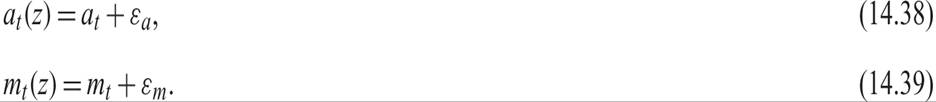
For simplicity, and without significant loss of generality, we shall assume that both the aggregate and the island-specific components are white noise processes. Thus, we assume that

where σ² denotes the variance of the aggregate component, and τ² is the variance of the island-specific component.⁸

Because all households face the same economywide price level for their consumption bundle and the same nominal interest rate, at the end of the period, they will all choose the same level of consumption. The price level, aggregate consumption, and aggregate output will thus be determined by

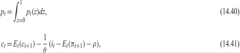
respectively. This completes the presentation of the model.

14.3.2 The Determination of Output and Employment

Under the assumptions we have made, output and employment on each island are determined on the basis of local information only. Aggregate consumption and the nominal interest rate are determined on the basis of full information at the end of the period.

Equating labor supply (14.34) and labor demand (14.35) on each island, we get that employment is determined by

where = ln (1 − α).

Substituting the employment equation (14.43) in the local production function (14.36), we find that output supply is determined by

In (14.44), we have used (14.42) to write expected consumption in terms of expected aggregate output, because there is no investment in this model, and all output must be consumed. When aggregated across markets, (14.44) denotes a positive short-run relation between aggregate output and unanticipated inflation.

Equating (14.44) with local aggregate demand (14.37) and solving for the local price level, we get

Using (14.42) to substitute for expected aggregate output by expected aggregate real money balances m − p, we can rewrite (14.45) as

Equation (14.46) denotes the local price as a function of the exogenous processes for productivity and the money supply (real and monetary shocks), and the rational expectations of the price level and of the aggregate money supply on the basis of local information.

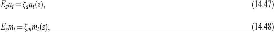
Given the assumption that productivity shocks and the money supply follow white noise processes of the form of (14.38) and (14.39), the rational expectations of aggregate productivity and the aggregate money supply, given local information, are determined by

where , and .

Note that in the case where there are no relative real and monetary shocks (i.e., when shocks are purely aggregate), , and it follows that ζ_a = ζ_m = 1. In this case, there is no confusion between aggregate and relative shocks, and we are back to the full-information new classical model of section 14.1.

Substituting (14.48) in (14.46), the equilibrium local price can be written as

Equation (14.49)—which expresses the equilibrium local price as a linear function of the expected aggregate price and the two exogenous shocks to productivity and the money supply—can be easily solved by using the method of undetermined coefficients.

14.3.3 The Real Effects of Monetary Shocks in a Rational Expectations Equilibrium

Let us assume that the solution for the local price takes the form

where the ψs are unknown coefficients to be determined. Then, given our assumptions, the solution for the aggregate price level is given by

From (14.51), the rational expectation of the aggregate price level given only local information is given by

Substituting (14.47) and (14.48) in (14.52), we get

Substituting (14.53) in (14.49) and rearranging, we get

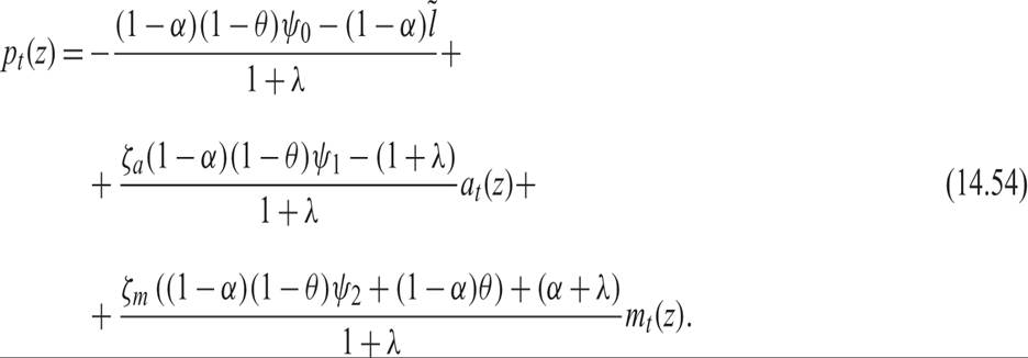
By comparing coefficients between (14.54) and (14.50), we can then determine the ψs as

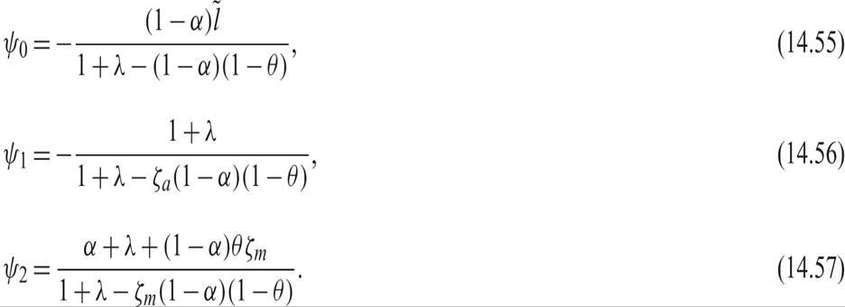
Note that in the case of perfect information, ζ_m is equal to unity, and ψ₂ is then equal to unity. The elasticity of the price level with respect to monetary shocks is equal to unity under full information. Under imperfect information, the elasticity ψ₂ is smaller than unity, as there is also a positive effect on real output, because of the confusion between absolute and relative changes in prices.

To solve for output, we can again use the method of undetermined coefficients. Let us assume that the solution for local output takes the form

where the γs are unknown coefficients to be determined. From (14.58), aggregate output is determined by

From (14.59), the rational expectation of aggregate output given local information is

From (14.50) and (14.53), the difference between the current local price on island z and the expected aggregate price level is given by

Substituting (14.60) and (14.61) in (14.44), the solution for output takes the form

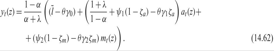
Comparing coefficients between (14.58) and (14.62), we find that

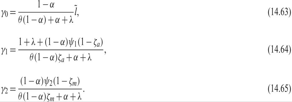
From equations (14.59), (14.63), (14.64), and (14.65), which describe the solution of the model for aggregate output, it is clear that both real and monetary shocks affect fluctuations in aggregate real output. The real effects of monetary shocks depend on ζ_m, the ratio of the variance of aggregate monetary shocks to the variance of both aggregate and relative monetary shocks. Monetary shocks have real effects in this model, because ζ_m is less that unity (i.e., because they cause a confusion between purely nominal and real fluctuations in real wages).

A positive monetary shock causes an increase in both the price level and nominal wages. However, because of imperfect information about the price level, workers rationally attribute part of the increase in the price level to an increase in the relative price of goods on their own island. Hence, they overestimate their real wage, they supply more labor, and employment and output increase. Because of imperfect information, monetary shocks thus have temporary real effects.

These real effects are transmitted to all real variables: employment, real wages, and the real interest rate. Combining the solution for output with the rest of the model, it is easy to show that these real variables are all affected by monetary shocks. The relevant solutions utilizing the rest of the model are given by

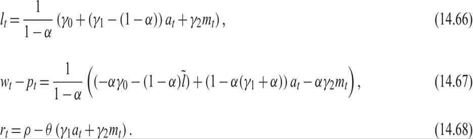
One can see from (14.66)–(14.68) that because of imperfect information, monetary shocks also cause fluctuations in employment, real wages, and the real interest rate. Thus, monetary shocks have temporary real effects across the board.

A positive monetary shock causes an increase in prices and nominal wages, but also an increase in employment and output and a reduction in real wages and the real interest rate. The reduction in real wages causes firms to increase employment and output. However, because households underestimate the increase in the price level, they supply more labor, interpreting part of the increase in nominal wages as an increase in real wages. Real interest rates fall to induce households to consume the higher output.

Note that if households had full information about the price level and aggregate shocks, ζ_m would be equal to unity, and γ₂ would be equal to zero. In this case, there would be no real effects from monetary shocks, and we would be back to the model of section 14.1, where only productivity shocks affect real variables. The contribution of the Lucas [1972] imperfect information assumption is that it allows for a short-run nonneutrality of money in an otherwise purely new classical model of aggregate fluctuations.

14.3.4 Optimal Monetary Policy in the Lucas Model

Optimal monetary policy in the Lucas model would not differ from the case of the new classical model with perfect information. If the central bank completely stabilized inflation, households would not confuse relative and aggregate price movements, as they would be able to perfectly forecast the price level. Hence, the short-run trade-off between inflation and real variables would disappear, as inflation would be constant, and all real variables would be at their equilibrium levels. Therefore, optimal monetary policy would again be the Fisher rule of full inflation stabilization.

14.3.5 The New Classical Model and the Great Depression

The explanation of the positive short-run relation between inflation and output and employment offered by the Lucas model is in terms of intertemporal substitution in labor supply and unanticipated inflation. Thus, if it were to account for the Great Depression of the 1930s, it would attribute this event to an unanticipated contraction in the money supply, causing an unanticipated deflation and a rise in real wages, which resulted in lower employment and output. The reason that labor supply fell would be attributed to imperfect information by workers, who mistook the nominal wage deflation for a fall in real wages. The model would not be able to account for the rise in unemployment, unless the rise was interpreted as a temporary fall in labor supply.

In any case, the model would also have problems accounting for the persistence of the Great Depression, as only unanticipated shocks to the money supply have real effects in such a model, and the model would have to invoke a sequence of unanticipated negative monetary shocks.¹⁰

14.3.6 Models of Informational Frictions and Rational Inattention

The weaknesses of the original classical models based on misperceptions and informational frictions notwithstanding, there has been a recent revival of interest in such models. Mankiw and Reis [2002], Sims [2003], and Woodford [2003b] pioneered this revival by proposing new formalizations of informational frictions and arguing in favor of rational inattention by agents to informational frictions. See Angeletos and La’O [2009] and Machowiak and Wiederholt [2009] on recent attempts to explain business cycles in terms of such frictions. Angeletos and Lian [2016] survey this recent literature and its implications for monetary policy. These more recent models are more sophisticated than the original Lucas [1972] model, and some of them emphasize strategic interactions between agents with different information sets. Yet they rest on similar premises as the Lucas model, such as misperceptions of aggregate shocks and intertemporal substitution in labor supply.

14.4