B Probability from the Bayesian Perspective

The Bayesian notion of probability is poles apart from the frequentist one. It is subjective, not objective. An extreme statement of the Bayesian point of view² is that “Probability does not exist.” '1 hal is, probability is a purely abstract construct that has nothing to do with events that are external to us.

'1 he National Weather Service (NWS) calculates the chance of rain (the “prob­ability of precipitation”) as the degree of confidence that it has that rain will fall somewhere in the forecast area multiplied by the percentage of the area that will see rain.⁵ '1 he degree of confidence reflects the percentage of times the NWS was right in predicting rain on “days like tomorrow” without being too precise about what tomorrow will be like. And there are other ambiguities. While “rain” means at least 1/100 of an inch of water, the “forecast area” is not well defined. Hence, despite the formulas and numbers, weather forecasting exemplifies the subjec­tive Bayesian approach to probability. It entails a degree of belief in an outcome; a belief that is usually shaped by past experience, a mathematical model, or hard evidence of the probability of occurrence of similar events.

More pertinent for scientists is the concept that if you combine quantitative information with appropriate assumptions supported by available data, you can make a Bayesian subjective probability calculation that predicts the chance that a hypothesis is correct. You can immediately see the appeal of the approach. Rather than being confined to assessing the truth value of hypotheses indirectly by eliminating false ones and amassing tested-and-not-falsified ones—Popper's strategy—Bayesianism offers the prospect of directly assigning (probabilistic) truth values to hypotheses. The critical prior assumptions in the Bayesian method, universally referred to as priors, are expressed as numerical probabili­ties, or probability density functions (confusingly abbreviated pdfs). Much hinges on the validity of the priors. A Bayesian analyst typically begins by finding appro­priate priors to use in her calculations, so we begin by examining how priors are incorporated in a Bayesian-type problem.

6. B.1 A Bayesian Problem

Suppose you are researching the growing problem of prescription opioid addic­tion in the United States. While visiting your local addiction center to interview addicts, you discover that 90% of them, a probability of 0.9, use marijuana regu­larly. This is alarming, and you leap to the inductive generalization that regular marijuana use is a predisposing factor, a “gateway drug,” to opioid addiction. You vow to spearhead a massive anti-marijuana campaign. Luckily, just before you do, a statistician friend informs you that your reasoning is flawed.

In fact, you can't determine the relationship between marijuana use and opioid addiction from what you know. To decide whether or not it's time to ban pot, you have to answer the question: “What is the chance that a marijuana user will be­come an opioid addict?” In other words, you want to start with a group of people who are marijuana users and ask how many of them go on to become opioid addicts. This not the information that you got from the clinic visit. Instead, you learned about a group of opioid addicts who also use marijuana. Not the same thing at all, and you have to distinguish what you know from what you need to know. Besides the addicts who use marijuana, you need to know the chance (the prior probability) that a random person uses marijuana and the prior probability that a random person is an opioid addict. Once you have these data, then you can use Bayes’ Theorem, also called Bayes’ Rule, to put them together and figure out the chance that a marijuana user is also opioid addict, which is what you want to know.

The problem might sound complicated, but it is simple in symbols, or, if you prefer, a diagram (Figure 6.1). If we use M to stand for marijuana use and A for opioid addiction, then the probability that an opioid addict uses marijuana is p(M/A). This is the probability, p, that the condition to the left of the slash (uses marijuana) is true, given that the condition to right of the slash (is an opioid ad­dict) is true.

The expression p(M/A) is called a conditional probability because it is the probability of one condition occurring given that the other condition already

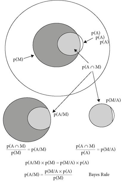
exists. This conditional probability p(MZA) is what you learned during the clinic visit. Its value is 0.9; however, what you're trying to find out is the probability that a marijuana user will become an opioid addict, denoted p(AZM).

At the other extreme from objective and informative priors are subjective and noninformative (or uninformative) priors. Noninformative priors are not based on experimental data. A noninformative prior might be a numer­ical constant or other estimate based on mathematical functions. If you didn't have the clinic data, you might have made the neutral guess that 50% of addicts would use marijuana, and then your estimate of the proportion of marijuana users who become opioid addicts would drop to 3%, half of what you previ­ously estimated.

Bayesians disagree about what is acceptable when it comes to subjective priors. The source of subjective priors ranges from plausible estimates to the quantifica­tion of expert opinion. For some Bayesians the concept that opinion alone could be a valid prior is a bridge too far; opinion, they believe, belongs to psychology. To someone raised with traditional frequentist sensibilities, formally including even expert guesswork into a quantitative equation is an odd way to proceed; on the other hand, if you recall that Bayesians equate probability with degrees of subjective uncertainty, then perhaps it is not so strange.

Sometimes people reveal their degree of confidence in a subjective probability prediction by placing a monetary bet on it. In fact, the ex-gambler, sports better, and professional election predictor Nate Silver¹¹ sees placing a money bet as the acid test of a prior. Because you care about the outcome—it's your money!—you have every incentive to evaluate the odds as rigorously and accurately as you can. The physicist Stephen Hawking once expressed $100 worth of confidence that the Higgs boson would not turn up in experiments done at the Large Hadron Collider and had to pay up when it did.¹² Hawking's experience highlights one of the dangers of subjective probability.

6. A.2 Bayesian Hypothesis Updating

Bayes' Theorem lets us estimate whether a given hypothesis is likely to be correct and, especially, to update and improve predictions as new information becomes available. To appreciate this feature of Bayesian reasoning, the first thing is to rewrite Bayes' Theorem in a general, scientifically relevant form. Typically, a Bayesian scientist would like to know how some data that he's gathered affect the chances that his hypothesis is true. That is, he wants to determine the hy­pothesis is true given the data—p(hypothesisZdata)—and to do that he needs to know the chance that he'd get that data if the hypothesis were true (i.e., p(data/ hypothesis)). Finally, he has to estimate the probability that the hypothesis is true in the first place, p(hypothesis) and the probability of observing the data, p(data) that he's gathered. With this information, he can use Bayes' Theorem like this:

^(hypothesis/ data ) = [ p( data/hypothesis) x p(hypothesis)] / p(data)

Equation 6.2

(Note that Equation 6.2 is just Equation 6.1 with new labels.)

Here's an example of how data can improve the probability that a hypothesis is true: imagine that you've made a new acquaintance, Pat, and, knowing nothing about Pat's occupation, you are curious (OK, nosy) about her salary. Knowing nothing, you can only assume that she is a typical member of the American work force and therefore that the odds of her earning less than $250,000 are 97 of 100 (97%).¹³ In other words, your best guess is that she makes less $250k a year; this is your initial hypothesis, so p(hypothesis) = 0.97. Subsequently, you learn that Pat has just bought a new sports car with a base price of $68,000. Immediately, you reeval­uate your image of Pat's resources, estimating that someone would have to earn at least $100k per year to be able to afford that car (in other words, buying the car is ev­idence that she makes >$100k). You want to know the probability that she can afford the car if she makes less than $250k.

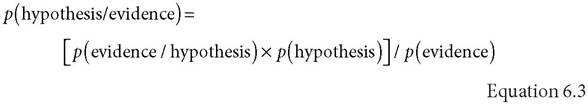
The answer is 82%, meaning that there is an 82% chance that she earns less than $250k a year. Thus, learning that she'd bought the car decreased your es­timate that she is in the under-$250k group of wage earners from 97% to 82%; still high, but lower than it was. Or, turning the numbers around, the chance that Pat makes more than $250k has jumped from 3% to 18%. You could continue the process if you got more information. If you learned that Pat is an analyst­level investment banker and that these folks make a minimum of $80k, with an average annual salary in the range of $120k—350k,¹⁴ you could further adjust your estimate. Now p(hypothesis) might be only 0.1 (10%), p(evidence/hypo- thesis) might go to 90% (0.9), and your estimate that she makes less than $250k would drop down to 45%. Progressively incorporating new information about Pat's circumstances would dramatically alter your hypothesis about her income.

Because you have to estimate priors, even “objective” ones, there is always an element of subjectivity in Bayesian probabilities. Even when based on previous evidence, subjective probability is a more flexible notion of probability than is frequentist probability because it depends on assumptions that are themselves uncertain. How accurate are the priors, and how applicable are they to the case at hand? Knowing her job description and its handsome salary range would still not tell you unequivocally how much money Pat makes—maybe she's an idealist who is just not that interested in making a lot of money, but a rich uncle died and left her a pile of cash and her lavish spending is entirely unrelated to her income. While Bayesian procedures give you a rational way of adjusting your confidence in your hypotheses, they also give you a way to compare hypotheses to find the stronger one.

6. A.3 Bayesian Hypothesis (Model) Selection

Frequentists test hypotheses (or “models”; we'll compare the two in Chapter 10.B) and reject improbable—effectively, falsified—ones. Classically, Bayesians don't reject hypotheses. The usual frequentist statistics compare a test result with an imaginary, idealized probability distribution to decide whether to reject their hypothesis or not. Bayesians think this makes no sense whatever.¹⁵ How, they ask, can you possibly arrive at valid conclusions by com­paring data that you didn't measure against a population that you can't ob­serve? Bayesians prefer hypotheses that postdict actual data already in hand, and they conclude that a superior hypothesis postdicts existing data with a higher probability than an inferior one. Otherwise said, they trust a hypothesis more if it has already performed well in the past, and they select hypotheses based on past performance.

Suppose you have two hypotheses, H₁ and H2, that can both account for ex­isting data, D, and you want to decide which one is best. You can assess their strengths using Bayes' Theorem (Equation 6.2) to calculate the posterior proba­bility of each H given D (i.e., [p(H/D)]). This tells you the probability that each hypothesis is likely to be correct given the data that you have. If H₁ predicts the existing data with a higher probability than H₂, then you conclude that H₁ is su­perior to H₂. In the usual notation, you set

against

p(H2/D) = [ p(D/H₂ )x p(H₂)] Ip (D) Equation 6.5

and choose the one with the higher probability. Alternatively, you can just divide Equation 6.4 by Equation 6.5, and if the result is >1.0, then H₁ is superior; if it is according to Miller's analysis, if Bayesians are truly inductivists, they cannot avoid the problem of induction. There is no guarantee that the future will be like the past. Therefore, he concludes that, to the extent that Bayesianism is deductive, it is not directly related to the search for Truth. To the extent that it is inductive, it suffers the weaknesses that cripple every other

bayesian basics and the scientific hypothesis 155

inductive method. Hence, for the Critical Rationalist, pure Bayesianism is nei­ther inductivist nor part of a quest for universal scientific Truth. It is simply irrel­evant to basic science.

But, we might ask, do scientists really have to choose between Popper and Bayes? Perhaps not, as I'll try to show in the next section.

6. D.1 Bayesianism and the Hypothetico-Deductive Method

Some Bayesians, including Andrew Gelman and Cosma Shalizi²⁴ consider the interpretation of Bayesianism as an inductivist procedure to be “faulty.” 'lhey think that, rather than incrementally increasing the strength of predictive models, Bayesians should pay more attention to active hypothesis “checking”; that is, testing and rejecting hypotheses in line with the traditional scientific modus operandi. For example, in studying the relationships among people's in­come and their voting behavior across states, Gelman and Shalizi carried out Bayesian-style hypothesis checking and correction to learn from more elabo­rate hypotheses what factors were most important for accurate prediction. The authors argue that “'1 he power of Bayesian inference here is deductive: given the data and some model assumptions, it allows us to make lots of inferences, many of which can be checked and potentially falsified.”

The prior distribution, in particular, is a testable component of a Bayesian inference process, and Bayesian hypothesis checking is like conventional frequentist-based, statistical testing of a hypothesis prediction. Gelman and Shalizi go on, “'1 he main point where we disagree with many Bayesians is that we do not see Bayesian methods as generally useful for giving the posterior proba­bility that a model is true, or the probability for preferring model A over model B, or whatever.” Rather, they argue, that “Certain of the model's implications [should be] compared directly to the data, rather than entering into a contest with some alternative model.... '1 he goal of model checking, then, is not to dem­onstrate the foregone conclusion of falsity as such, but rather to learn how this model fails.” And a model that has failed is a model that has been falsified.

Note that Gelman and Shalizi's suggestion for interpreting Bayesian procedures deductively is quite different from David Miller's. Miller focused on how Bayesians use Bayes' Theorem to reason about the probability that a hypo­thesis is true; Gelman and Shalizi propose that we should use Bayesian statistics to decide whether to accept or reject a hypothesis. Using Bayes' '1 heorem to test a hypothesis would be largely free of the criticisms that plague null hypothesis significance testing mode (NHST) procedures, for example, in the context of the Reproducibility Crisis (Chapter 7).

6. D.2 A Bayesian Standard for Falsification

'lhe potential for applying Bayesian methods to hypothesis testing evidently hasn't been exploited to any great extent, so I'd like to explore it a little more. Ordinarily, with Bayesian methods, you choose between two models by com­paring their posterior odds ratios and opt for the one with the higher posterior odds of postdicting the data already at hand. However, rather than concen­trating solely on the probabilities per se, as a pure Bayesian analyst would do, experimental scientists could simply agree on a quantitative standard for rejecting the weaker hypothesis. For example, following the reasoning in Box 6.1, we might agree that a Bayes factor of, say, 10, would be sufficient to declare the less probable hypothesis to be falsified (see example in Box 6.2). 'lhe critical value of the Bayes' factor would be a matter for each scientific com­munity to set, analogously to the present p < 0.05 level for rejecting a hypo­thesis. A methodological rule like this would allow Bayesian criteria to fit into a hypothesis-testing philosophy.

6. D.3 Bayes and Explanation

While we hope that good predictive models will have explanatory force, it is true that greater predictive accuracy does not imply greater understanding. You can make good predictions without good understanding, as the Ptolemaic and Mayan astronomical systems showed. It is not that predictive power is unimpor­tant in science; on the contrary, applied science, technology, and even basic sci­ence fields place high value on accurate predictive hypotheses. It's just that basic science is not ultimately satisfied with better predictive hypotheses unless they are primarily explanatory.

6.