Four Scenarios

In order to exemplify the simulations, four scenarios with a configuration as described in Table 9.4 are presented in the Figs. 9.4, 9.5, 9.6 and 9.7, which show the simulations 20 years after the start (i.e.

in the year 3980 BC). In order to highlight the implications of the cropping systems, the other parameters are unaltered or vary only to a minor extent. The model allows for any of the parameters in Table 9.4 to be changed, so the scenarios shown here represent only a few out of 320 possible configurations. The main window shows the landscape development due to the processes performed by the inhabitants of the households. In the upper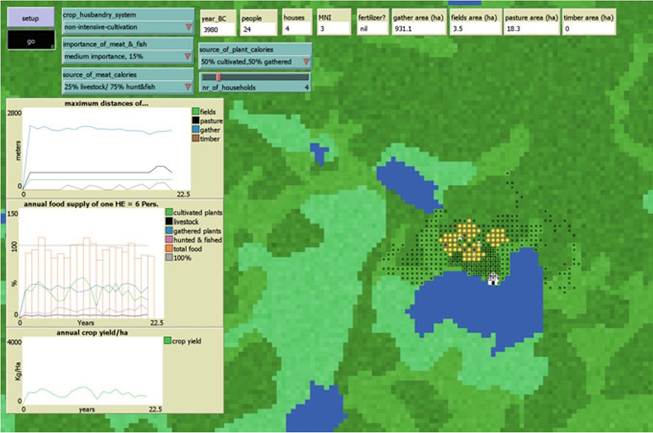

Fig. 9.5 Scenario 2 simulating land use, resource use and economic parameters of a hypothetical Neolithic wetland settlement relying on non-intensive cultivation. Black boxes are patches affected by timber extraction. The other symbols have been described in Fig. 9.4

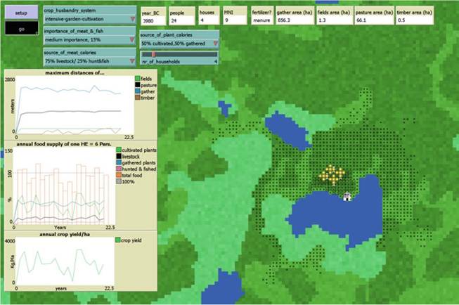
Fig. 9.6 Scenario 3 simulating land use, resource use and economic parameters of a hypothetical

Neolithic wetland settlement relying on IGC. All symbols have been described in Figs. 9.4 and 9.5

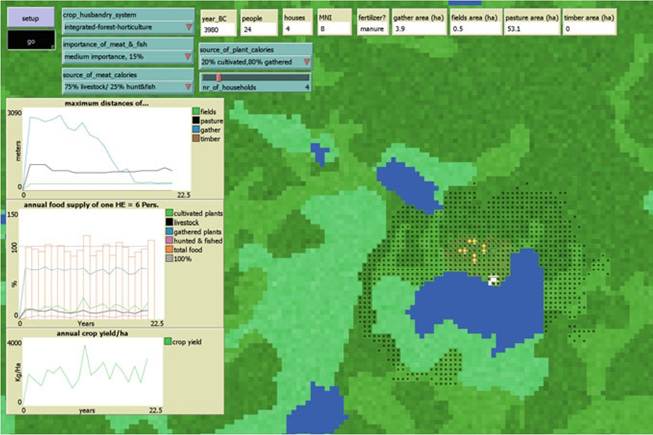
Fig. 9.7 Scenario 4 simulating land use, resource use and economic parameters of a hypothetical

Neolithic wetland settlement performing IFH. All symbols have been described in Figs. 9.4 and 9.5

Table 9.4 Specifications of the Scenarios 1-4 as shown in Figs. 9.4, 9.5, 9.6 and 9.7 and discussed in the text. Abbreviations as above

	Cropping system	Importance of animal products	Source of plant calories	Source of meat calories
Scenario 1	SC	“Medium (15 %)”	“50 % cultivated, 50 % gathered”	“25 % livestock/75 % hunting and fishing”
Scenario 2	NIC	“Medium (15 %)”	“50 % cultivated, 50 % gathered”	“25 % livestock/25 % hunting and fishing”
Scenario 3	IGC	“Medium (15 %)”	“50 % cultivated, 50 % gathered”	“75 % livestock/25 % hunting and fishing”
Scenario 4	IFH	“Medium (15 %)”	“20 % cultivated, 80 % gathered”	“:75 % livestock/25 % hunting and fishing”

left corner, model parameters can be specified.

The small white boxes on the upper rim show details of the actual model status. On the lower left side of each of the panels, three monitors are located. The upper one shows the annual maximum distances for the economic activities of the settlers as conditioned by the model parameters. The panel in the center shows a graph where the annual food supply is plotted. Lines of different colors give the annual supply of the different categories adding to the calorie supply, while red bars show the total provisions in relation to the aim (=100 %), which may or may not be met due to stochastic factors of food production.

The lower panel displays the annual crop yield given in kg/ha, which is dependent on weather variability, soil fertility and the chosen cropping system. In each scenario, 24 persons in 4 households perform land and resource use in order to meet their requirements. The proportion of animal products is 15 % in all scenarios, while the cropping systems and the composition of the vegetal and the animal shares vary. Scenario one (Fig. 9.4) shows the application of SC. This practice allows for high yields per ha with a maximum of 4330 kg/ha in year 20 and thus, individual field size per year need not be large. Each household unit is burning and cultivating only 5 patches (yellow field symbol) equaling less than one third of a hectare. Altogether, the four households require an area of 1.3 ha to produce enough crop plants to cover (100 — 15)/2 = 42.5 % of their calorie demand (see Table 9.3). However, due to the additional forest area required to gain wood suitable for this specific burning procedure, large areas are affected in the course of twenty years. This is depicted by the brown patches symbolizing fallowing areas due to prior field use or forest cutting. As large forest areas are cleared annually, I assume that no additional areas for timber extraction are required. The fallowing areas provide possibly a very good livestock pasture, and only a small area is needed annually for this use category.

Similarly, the growth of wild food plants such as berries, apples and especially hazelnuts is strongly stimulated on fallows of a certain age. Even when no direct anthropogenic promotion of these plants is assumed, the area necessary to cover a relevant proportion of the calorie demand by gathering is relatively low when the hazel bushes reach a certain age and start bearing nuts. Hazelnut—bushes need a few years to establish, and only from their 5th year on will they produce an annually increasing harvest of nuts in WELAS- SIMO. In year 15, they reach their maximum harvest potential and hold this for 35 years. In the upper panel of Fig. 9.4, the decreasing distances for gathering activities are observable. Pasture distances decrease less pronounced, as the difference in fodder—value between primary forest and fallowing land is not as large as in gathered human foodstuff. Additionally, the effect is masked by the low MNI and the large fallowing area from year two on. The farthest distance of economic activities is about 1000 m after twenty years, and the reason for this distance is the high land demand for SC. As can be seen in the center panel, food requirements are met in 9 years out of twenty. This is however not related to the cropping system, but is due to the built-in stochasticity of yields due to weather variability simulated by the model. A bad series of low crop yields occurs in years 1 and 2 and in the years 14 and 15 of the simulation. In WELASSIMO, this has no consequences for the settlers, as an assessment of the consequences of food shortages and demographic implications are not the aim of this research.

Scenario two shows the situation for NIC (Fig. 9.5). All model parameters except the cropping system are the same as in Scenario 1. As no fertilizing occurs, annual yields are quite low with a maximum of 1050 kg/ha in year 10, and nutrient depletion further affects the crops as cultivation duration increases. 14 patches are needed per household, equaling 3.5 ha for the four households.

Successively, the households will relocate the fields when a certain threshold of soil fertility is reached and yields begin to decrease largely. Only a few fallowing patches are seen bordering the fields. As most other areas are primary forest, which is relatively low in animal fodder, a larger area than in scenario 1 is needed for the feeding of the livestock. The same holds true for wild edible plants, so in order to cover the same proportion of calorie demand from wild plants as in the SC scenario, a much larger area is needed (931 ha in comparison to 4.8 ha). Black boxes around patches in Figs. 9.5 and 9.6 symbolize areas affected by timber extraction. In the course of time, the distances for this activity increase, as nearest suitable trees to the settlement are felled first and more distant ones later. After 20 years, the distance to meet the demand in suitable construction timber has reached 200 m for the 4 households. The distance to the other economic activities does not change to a large extent in the course of time. The calorie requirements are met in 9 out of 20 years. In year 12, a bad crop yield occurs, and only 78 % of the food provisions are acquired.

Scenario three (Fig. 9.6) depicts the situation for IGC. All model parameters remain the same as before, except the source of meat calories as described below. Due to intensive weeding and manuring, permanent fields cultivated for several years may be assumed without relevant soil nutrient depletion. Field sizes are quite small due to relatively high yields per ha (avg. 2400 kg), and 5 patches equaling a third of a hectare are sufficient for one household. The fact that the number of patches for crop husbandry are the same as in scenario 1 is due to rounding of decimal places in the model; exact numbers differ, but this is not shown. The high manure application necessitates a quite large MNI (Minimal Number of Individuals, i.e. livestock). This is automatically accounted for inside the model script when IGC or IFH are selected; to highlight these relationships, I have raised the share of livestock for the supply with animal products (which remains medium = 15 %) deliberately to 75 %.

The high MNI require a large area annually for forest-grazing and pollarding. As already discussed above, primary forest is lower in livestock fodder; thus in scenario three, very large areas are needed to feed the livestock. Yet similar as in scenario 2, the largest area is needed for gathering wild edible plants. While the distances of fields and pastures remain more or less stable, the need for suitable timber constantly leads to more distant timber areas as already shown in scenario two. The calorie requirements are met in 7 out of 20 years only, with a remarkable depression in calorie supply in the years 10-13—but again, this is not reflecting any other factor than the built-in stochasticity of yields due to weather variability.

Scenario four simulates the application of IFH. The source of calories of animal origin is 75 % livestock and 25 % hunted, as in scenario 3, but in contrast to the other scenarios, only 20 % of the vegetable calories are covered by crop plants, while 80 % are collected, the bulk of which is assumed to be hazelnuts. This represents the hypothesis that the well-documented hazel and charcoal peaks in the pollen profiles might rather reflect the use of fire for the opening and shaping of the vegetation cover, than being coincidental side-effects of SC. As the benefit of these measures would not only be the promotion of hazel growth, but as well good livestock browsing and presumably higher numbers of suitable timber than found in primary forest, the necessary zone of land-use activities may be smaller than in the

Table 9.5 An overview of the maximum distances for economic activities for a simulated settlement size of 4 households (=24 persons) as a result of WELASSIMO

Scenario	5 years, 4 households	20 years, 4 households
1	2.2 km, gathering	1.0 km, fields
2	2.0 km, gathering	2.0 km, gathering
3	2.1 km, gathering	2.1 km, gathering
4	2.8 km, gathering	0.7 km, pasture

previous scenarios.

This effect will show after a few years of cultivation, as can be seen in the upper graph of Fig. 9.7. In the beginning of the simulation, when no nut-bearing hazel bushes exist, the high proportion of gathered calories causes a large radius for gathering activities (note the maximum value on the y-axis, which is different from the other three scenarios). After a couple of years, however, this distance is reduced drastically, and then the most distant activities are livestock browsing in 740 m distance—thus, IFH allows for the smallest economic area of all scenarios. The annual opening of new fields for the creation of new “forest gardens” is assumed to cover the need in timber, thus no extra area is needed similar as in scenario 1, and in contrast to scenarios 2 and 3. As intensive cultivation of the fields is assumed here similar to IGC, and due to the low proportion of cultivated plants, only two field patches per household are sufficient, which is equivalent to an eighth of a hectare per household or 0.5 ha for 4 households An MNI of 8 heads of livestock for the settlement results out of this configuration. The calorie requirements are met in 18 out of 20 years, with a set of bad harvest in collected plants paralleled by low crop yields in the years 5 and 6 of the simulation. Annual variation in the harvest of gathered plants is assumed to be less fluctuating than for crop yields, which is discussed below; the effect of this hypothesis is less variation and less pronounced extremes of food supply. This is especially evident in year 10 of the simulation, where a remarkable peak in crop yields of 3570 kg/ha results only in a minor over-achieving of the total provisions. Table 9.5 gives an overview of the maximum distances for economic activities resulting out of different configurations after 10 and 25 years of simulation for the scenarios described above.

9.6

<< | >>

↑

Source: Barcelo Juan A., Del Castillo Florencia (eds.). Simulating Prehistoric and Ancient Worlds. Springer,2016. — 410 p.. 2016

Four Scenarios

More on the topic Four Scenarios: