Chapter 63 Does Geography Matter? A Study of Determinants of Bank Office Size in Illinois
Bin Zhou
Southern Illinois University Edwardsville, USA
ABSTRACT
This study investigates the role of geography in shaping the average bank office size in Illinois banking.
“Geography” here refers to a host of socioeconomic, demographic, and local community characteristics at the bank market level. The study finds that larger bank markets, higher levels of market concentration, higher percentages of whites within the total population, and less physical fragmentation within a geographical bank market contribute to larger average bank office sizes. The use of technology, represented by higher percentages of physical capital and premises in the total assets, is found to reduce the bank office size. This tendency is further reinforced by a lack of economies of scale at the bank office level. At the same time, the study finds that the greater adoption of internet banking is associated with larger bank offices. These findings provide indirect evidence that market structure has an impact on the adoption of alternative banking technologies. A study of bank office size has practical implications in providing insights into the future branch strategy, as well as the inadequate nature of measures of market power currently used in antitrust regulation.INTRODUCTION
This study investigates the role of local socioeconomic, demographic, and community factors as determinants of bank office size, along with the role of technology, economies of scale, and bank market conditions that have long been recognized as factors in shaping bank office size. Over the past thirty years, the U.S. banking industry has undergone significant restructuring. Three areas of
DOI: 10.4018/978-1-4666-6268-1.ch063
restructuring can be identified: banking consolidation and institutional changes, portfolio changes and product and service diversification, and geographical deregulation in the form of nationwide interstate banking and branching.
In light of the 2008-2009 financial and banking crisis and current economic difficulties, the merit of these transformations is called into question. Nonetheless, given the changes that have already taken place, studies on characteristics of banking structure can still provide valuable insight into the state of the U.S. banking industry. One particular facet of banking structural change is bank office size. As banks in the United States become increasingly large, the average size of bank offices becomes increasingly small (Hannan & Hanweck, 2007). In addition to a drastically changed regulatory environment, overall banking consolidation, and adoption of the latest technologies, changes in bank office sizes may have also been associated with locally based conditions, which can be collectively subsumed under “geography.”Important geographical factors include the size of bank geographical markets, market structure, the physical configuration of local communities within a market, local ethnic composition, per capita income, population density, level of urbanization, level of education, characteristics of the local economy and the local banking industry, etc. Although market structure, economies of scale, and bank market conditions have long been recognized as contributing to the bank office size, other factors have yet to be adequately analyzed for their potential roles in shaping bank office size. This paper intends to fill this void, using Illinois banking as a case study..
Focusing on Illinois banking is of particular significance. As a traditional unit banking state where banks were prohibited by law to open branch offices outside their head offices, branch banking in Illinois has undergone dramatic development and the average size of bank offices has experienced constant changes since the banking geographical deregulation, making them one key area of structural change in Illinois banking. To understand structural changes in Illinois banking is in part to understand changes in branch banking and bank office sizes.
In contrast, in states such as New York where branch banking was allowed historically, branch development and changes in office size have not been a significant issue since banking deregulation. For example, between 1980 and 2007, while the number of commercial bank offices in New York increased by 4%, the same time span saw an increase of over 180% in bank offices in Illinois. As a result, 64 out of 84 (76%) Illinois banking markets experienced a decline in the average office size, while only 10 out 33 (30%) banking markets in New York did so.A study of determinants of bank office size has practical implications for the banking industry in general. As bank office size and banking at bank offices experience dynamic changes in part driven by banking technologies, the future branch strategy and the related bank office design have become important issues within the banking community. A study of geographical factors of bank office size may provide additional insight into the issues. In addition, the rising number of bank offices improves customers’ accessibility to bank services and reduces the market power exerted by banks within the spatial market. This calls into question the measures of market power currently used in antitrust regulation, which take into account the firm level market shares but leave out characteristics of branch banking and community configuration within a bank market. Arguments can be made for the need for more inclusive measures.
THE LITERATURE
A traditional perspective relates the bank office size to economies of scale at the bank office level. While some find significant economies of scale at the branch level (Longbrake & Haslem, 1975; Zardkoohi & Kolari, 1992), Nelson (1985) finds that branches display constant returns to scale up to the $20 million deposit size level, followed by increasing returns to scale after that. Benston, Hanweck, and Humphrey (1982) observe that average branch size stabilizes at the $25 to $35 million range and that further banking growth is more likely to be accommodated through opening new branches.
To a certain extent, the notion of economies of scale is related to the “optimal” level of resource deployment at the bank office, alluded to by Nas, Ray, and Nag (2005). They find that the personnel cost efficiency at the branch office level is in part related to the branch office size, and that the medium-sized offices have lower cost efficiency than small and large-sized offices. That is, the cost curve at the branch office level is reverse U-shaped. They also find that labor productivity is lowest at the smallest offices. As a result, consolidation of these offices would generate more productive offices through economies of scale.With the U.S. banking industry undergoing significant structural changes in recent decades, attention has shifted to the role of structural factors in shaping branch banking and thus bank office size. A number of authors point out paradoxical roles of technology in branch banking in recent decades (Hirtle, 2007; Nam & Ellinger, 2008). On the one hand, the technological advances such as ATMs, internet banking and electronic delivery, and centralized call centers have diversified the delivery of, and lowered the cost of, banking services. The traditional “brick and mortar” bank offices, as a relatively expensive channel of delivering banking services (Orlow, Radecki, & Wenninger, 1996), seem at a disadvantage. On the other hand, as shown previously, there has been a steady growth of branch bank offices in the United States since the 1980s (Nam & Ellinger, 2008). Despite the rapid adoption of technologies in banking, the need for bank offices has not disappeared.
Indeed, Spieker (2004) believes that branch offices are still a highly effective and profitable distribution channel for retail banking compared with internet banking and call centers. Some researchers note that neither ATM nor online banking provides full service banking, especially with regard to lending. Thus they are at present a service enhancement to conventional bank delivery, a supplement to the bank office, rather than a substitute (Brevoort & Wolken, 2008).
With changing technologies, the transaction mix at bank offices is changing too. The reduction in check- related transactions at bank branches is being replaced by the marketing of certificates of deposit, personal and commercial loans, mortgages, and credit cards (Contributor, 2009). There are still over 80% of bank customers who use an office once a month and 30% use an office 4 to 5 times each month (Wall Street Journal, 2003). Building branches has been one of the most effective ways for banks to compete for retail customers in recent years (Hirtle & Metli, 2004). Bank offices still matter in retail banking.Hannan and Hanweck (2007) report a general trend of declining average bank office sizes since the late 1980s, with the office size being measured by the average number of bank employees per office. Indeed, for the U.S. commercial banking industry as a whole, the average number of employees per bank office was 27 in 1980. In 2009, it was 21. Hannan and Hanweck attribute the office size reduction to technological factors such as the use of ATMs, which substitute for expensive bank tellers and results in smaller office sizes. They also see in-store bank offices as a broadly defined technological change causing the bank office size to be small. They also find that markets experiencing greater growth in branch offices experience greater reduction in the average size of bank offices. They take this as evidence that new technology may help reduce office size since in markets with faster office growth, new offices are more likely to incorporate newer technologies than old offices. They further speculate that with fewer numbers of employees needed to handle the operation of a branch, a larger number of smaller branch offices in a market becomes desirable. Hannan and Hanweck’s conclusions are important in providing insight into the role of new banking technologies. That is, although the latest banking technologies may not eliminate the need for, or reduce the number of, bank offices, they cause the bank offices to become smaller.
In other words, there is a substitution of technology for office size, rather than for the number of bank offices. Lower banking cost may come as a result of building smaller bank offices, rather than eliminating offices altogether.Among conditions that prevail at the local geographical level, market structure has long been recognized as contributing to bank office size. For example, Rice and Davis (2007) attribute changes in branch banking to the changing market structure and find that market structure becomes more competitive in cities experiencing rapid growth of branch offices. This is conceivable when many banking institutions engage in active branching. Since rapid branch building is also frequently associated with steady decline of the bank office size (as discussed later in the case of Illinois), Rice and Davis essentially associate competitive markets with smaller average size of bank offices. On the other hand, Avery, Bostic, Calem, and Canner (1999) find that mergers of banking networks with overlapping market areas may lead to the reduction of bank offices when the post-merger institutions consolidate the banking network within a market. Closing branches while maintaining the same volume of business may cause the average bank office size to rise. Kim and Vale (2001) point out that banks act strategically in their branching decisions, taking into consideration the future response by rival banks within the same geographical market. This leads to a situation where in a more concentrated market, banks are sensitive to actions from rival banks, thus may show restraints in branching. Increasing the size of operation at an existing branch may be a preferred or less provocative option. Indeed, Hannan and Hanweck (2007) find that at least in rural markets, more concentrated markets tend to be associated with large office sizes.
In discussing retail banking, mention should be made of central place theory pioneered by German geographer Walter Christaller and further developed by German economist Augusta Losch (Lloyd & Dicken, 1977), and more recently by Berry and Parr (1988), among others. Central place theory studies the relationship between the size of places and their functions, and the spacing between places of various sizes and functions. Although the size of establishments is not the central focus, it is nonetheless alluded to through notions such as range and threshold. The former refers to the maximum distance a customer would travel to purchase a service while the latter is the minimum aggregate demand (measured by population, customers, etc.) necessary for a firm to stay in operation (Lloyd & Dicken, 1977). Thus threshold provides a reference to the low bound of firm size while range defines the physical size of a firm’s market area. In the context of retail banking, it is conceivable that the traditional restrictions on branch banking would cause a bank office to serve a market significantly larger than its threshold, but force many customers to travel a distance close to their ranges. Branch restrictions were intended to protect the interest of local banks while the interests of consumers and the overall economy were inadvertently sacrificed (Calomiris, 2000). Indeed, studies find that traditional unit banking and restrictive branch regulations caused lower numbers of bank offices on a per capita basis than otherwise at both the county (Guttentag & Thomas, 1979) and state (McCall, 1980) levels. On the other hand, Dick (2003) finds rising branch density as a result of nationwide branching. Zhou (2010) finds Illinois, as a unit banking state, traditionally had a level of geographical concentration of bank offices much higher than the concentration of population, indicating a high degree of supply-demand mismatch. However, bank office concentration, along with the supply-demand mismatch, has drastically decreased amid geographical deregulation and rapid branch expansion over the last three decades (Zhou, 2010).
An important insight from central place theory is that service functions found at different places are associated with the size of places, with basic functions being available at both small and large places, and specialized functions available only in large places. Basic functions have lower thresholds which can be easily met in both small and large places. In comparison, specialized functions have higher thresholds and thus can only be met in large places (Berry & Parr, 1988). A connection is clearly seen between the size of places, the degree of specialization of functions, and the low bound of firm sizes. Holmes and Stevens (2004) drive this notion home by associating higher levels of specialization in services with larger plant size of service firms. Thus there is the logic of large market - higher end and specialized service - large office. This logic conceivably applies to banking, though there has not been any efforts seeking to prove such a connection in recent banking study.
THE ILLINOIS BANKING
For a long time, Illinois had one of the most restrictive branch banking laws in the United States (Rice & Davis, 2007). In 1870 the Illinois constitution declared Illinois a unit bank state. For the next one hundred years, most banks in Illinois remained unit banks. For example, in 1966 while a quarter of banks in the United States had branches, only 0.4% of Illinois banks did. A change came in 1967 when Illinois permitted a drive-in facility within 1500 feet of a unit bank. In 1970 when the state re-wrote its constitution, the prohibition on branch banking remained. In 1976, the state allowed a bank to establish a second facility within 3500 yards of the bank. Regional recession and a banking crisis in the 1980s forced the state to speed up banking deregulation. In 1982, a third “community service facility” within the same county was allowed. In 1985 up to 5 facilities or branches were allowed for a bank with the first facility being within 500 yards of the main bank, the second within 3,500 yards, and the remaining three within the same county. A branch could be located outside the county if it was within ten miles of the main bank. In 1987, prohibition of branch banking was formally repealed. However, restriction on branching died hard. Even in 1990, the state still set a limit of up to 10 branches in the home county, 5 in each contiguous county, and 5 in any other county within 10 miles of the main banking premises, though branching through mergers or acquiring troubled banks were not restricted. In 1993, the state finally allowed statewide branching without limitations on location or number.
Since the geographic deregulation, branch banking has become one of the most prominent developments in Illinois banking. Table 1 summarizes selected facts that reveal changes in the Illinois economy and banking, in comparison with those in the U.S. from 1980 to 2008. As can be seen, although increasing in population, real income, and deposits, the most dramatic growth in Illinois is that of branch offices with a 702% growth between 1980 and 2008 compared with 113% for the U.S. as a whole. For the U.S., the average number of bank office per 10,000 people barely changed from 1980 to 2008. For Illinois, the average number of bank offices per 10,000 people rose from below the national average in 1980 to above the national average in 2008. The ratio of the percentage of unit banks to the percentage of branch banks in Illinois changed from significantly larger than that in the U.S. in 1980 to a level comparable with the national average. From the last two rows of Table 1, it is clear that although increasing significantly, the average size of the branch banking network in Illinois still lags behind the nation.
The above comparison indicates important characteristics of change in Illinois banking. Branch banking has been a key development in Illinois during the past thirty years, after being shackled by the state law and regulations over a century. However, in understanding the nature of branch banking expansion in Illinois, it is necessary to go beyond the general interpretation of these developments as a response to fundamental geographical deregulation. Branch banking in Illinois is most likely uneven and responding to varied local dynamics in terms of socioeconomic, market, and community conditions. As rapid branch banking development has come only in recent decades and
Table 1. Selected facts of changes in banking: Illinois vs. the U.S.
| Illinois | U.S. | |
| Bank Branch Growth: 1980 - 2008 | 702% | 114% |
| Real Bank Deposit Growth: 1980 - 2008 | 8% | 142% |
| Population Growth: 1980 - 2008 | 13% | 34% |
| Real Personal Income Growth: 1980 - 2008 | 99% | 136% |
| Average Number of Bank Offices per 10,000 People: 2008 | 3.75 | 2.95 |
| Average Number of Bank Offices per 10,000 People: 1980 | 1.56 | 2.34 |
| Percent of Unit Bank vs. Percent of Branch Banks: 2008 | 26% vs. 74% | 25% vs. 75% |
| Percent of Unit Bank vs. Percent of Branch Banks: 1980 | 67% vs. 33% | 47% vs. 53% |
| Average Number of Branches per Bank: 2008 | 8.5 | 12.6 |
| Average Number of Branches per Bank: 1980 | 1.4 | 3.7 |
Sources: Calculated from the FDIC data.
is still ongoing, Illinois banking offers a fresh case study opportunity for researchers to investigate how a variety of current and prevailing local conditions, rather than historical inertias, have helped shape bank office size.
METHOD, VARIABLES, AND DATA
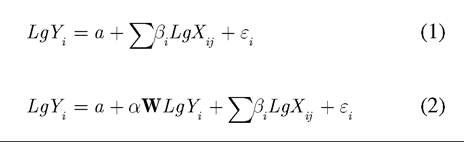
Following Hannan and Hanweck (2007), a multiple linear regression model, as shown in Equation 1, is used. In the equation, the dependent variable Yi is the average bank office size, while independent variables, X.. are a vector of determinants 1...j. Equation 2 is an alternative, spatial autoregressive model, which adds a spatial lag, WlgY to the original Equation 1, with W being the first order continuity matrix (Anselin, 1993), entries of which are binary values with Wij being 1 when two geographic markets are adjacent and 0 otherwise. The reason for a potential need for a spatial autoregressive model is that the observations used in the study are geographic markets in Illinois. Among spatially adjacent markets there may exist spatial autocorrelation. That is, the office size of one market may be influenced by those in neighboring markets as a result of operating in similar geographic areas or under a similar business environment. If statistical tests point to the existence of significant spatial autocorrelation, the spatial autoregressive model should be used. This is similar to a regression that uses time series data and thus needs to incorporate a time lag to account for possible serial correlation. In Equation 1 and/or Equation 2, a, α and βi are parameters to be estimated, and ε. is an error term:
l
An important departure from Hannan and Hanweck (2007) is that this study adopts deposits as a measure of bank office size, rather than using the number of employees. Hannan and Hanweck estimate the average number of employees per bank office by using data from County Business Patterns. County Business Patterns reports the number of bank offices falling within size categories such as 1-4 employees, 5-9 employees, 10-19 employees, 20-49 employees, 50-99 employees, 100-249 employees, etc. They estimate the total number of employees working in a particular size category by multiplying the mid-point (or the mean of the
lower and upper bound) of the size category (e.g. 2.5 for 1-4 category, 7 for 5-9 category, etc.) with the number of bank offices in that size category. For example, in 2008, 6 bank offices in Madison county, Illinois fell in the 1-4 employee size category. The total number of employees working in bank offices of that size category would be estimated to be 2.5 ?6= 15. Applying this method to all size categories would produce an estimated total number of commercial bank employees in a county. Dividing this number by the total number of bank offices in the county gives the estimated average number of employees per bank office in the county. Such estimation can be done for rural bank markets (non-metro counties) as well as the metropolitan markets.
The Hannan and Hanweck estimation method assumes an identical number of offices of various sizes within a size category. For example, within the size category 1-4, for the estimation to be accurate, there should be equal numbers of firms with one employee, two employees, three employees, and four employees. When this assumption is not met, distortion will occur. The amount of distortion can be demonstrated to be N?R∕2, where N is the number of offices within a particular size category and R is the width of a size category (difference between the upper and lower bounds). The details in deriving this expression of distortion and a graphic demonstration can be found in the Appendix. In general, the extent of distortion will rise with the number of offices within a size category and with the office size category.
As stated earlier, the present study adopts deposits as a measure of the bank office size. The amount of financial resources, such as asset or loan or deposits, has always been used as measures of the size of banking institutions. In examining economies of scale at the bank office level, Han- weck and Humphrey (1982) and Nelson (1985) use deposits as a measure of bank branch sizes. Distinction can be made between bank outputs and bank inputs (Gandhi & Swizter, 1988; Das, Ray, & Nag, 2005), with assets, deposits, lending, mortgages, total bank credits, etc. being bank outputs while staff members, equipment, office space, etc. are bank inputs. As a result, the bank office size can be alternatively measured using outputs or inputs. Hannan and Hanweck (2007) adopt an input measure of the bank office size while the present study uses an output measure of bank office size. The advantage of using deposits as a measure of office size is the data availability through the FDIC Summary of Deposits data. Under certain circumstances, input and output measures of office sizes may be consistent. For example, in Illinois, the average bank office size measured by the number of employees and that measured by the amount of deposits declined in lockstep from 1980 to 2009, leading to a correlation coefficient of 0.89.
In the Hannan and Hanweck (2007) estimation, the vector of independent variables includes local socioeconomic conditions such as population, per capita income, profitability measured by the rate earned on interest bearing assets, market concentration, immigrants, traffic congestion, and a dummy variable for intrastate banking deregulation. The present study adopts a more comprehensive set of independent variables fully represent local as well as general conditions. These variables can be divided into several categories. The first category includes socioeconomic variables within a local bank geographical market such as per capita personal income (PCI), the percentage of whites in the total population (WHITE), the percentage of population aged between 16 and 21 who are enrolled in public schools (SCHOOL) and the percentage of population aged between 18 and 65 (LABOR). Although these socioeconomic variables have not been widely adopted as bank office size factors, there are reasons to examine their potential roles. In terms of income level, it is conceivable that wealthy markets generate more deposits and thus demand for more sophisticated financial services, which tend to be associated with large bank offices, everything else being equal. The level of school enrollment is closely associated with the general level of education, which may affect the adoption of technologies in banking. More educated customers are more likely to adopt latest banking delivery technologies than the less educated. Similarly, of all adult bank customers, those still in the labor force are more likely to be open to the latest technology than retirees. Thus through their effects on using the latest banking technology, both more educated and active working customers would be associated with smaller bank office sizes.
The above hypotheses are supported by many surveys concerning consumer banking behaviors. Surveys by the American Bankers Association, a trade group, consistently find that younger age groups are more likely to use internet banking than older age groups (ABA Banking Journal, 2011). Surveys by the Federal Reserve Bank of Boston on consumer payment methods also reveal that when comparing the likelihood of adopting online payment among various socioeconomic groups, Asians and whites are more likely than African Americans and Hispanics to adopt these methods; high income-high net worth groups are more likely than lower income- lower net worth groups to adopt online payments; more educated groups are more likely than less educated groups to do the same (Schuh & Stavins, 2008). In addition, there is a large body of literature devoted to the issue of discrimination in banking against racial minorities (Bradbury, Case, & Dunham, 1989; Canner & Smith, 1991; Holmes & Horvits, 1994). To the extent that discriminatory practices are widespread, we would expect a smaller amount of resources available to banking, thus a smaller average bank office, in markets with higher racial minorities. In the years leading up to the 2008-2009 financial crisis, some banks aggressively expanded into sub-prime products serving the needs of lower income and/or racial minority populations. If such efforts led to rapid office expansion, they would act as additional contributing factors for smaller office sizes.
The second category of independent variables reflects the economic characteristics of the local bank markets. Banks serve consumers as well as businesses. Banks are always seen as the major source of financing for small businesses (or firms with employees under 500, a criterion set by the U.S. Small Business Administration except some manufacturing sectors for which the standard goes beyond 500). For example, the latest Survey of Small Business Finances, conducted in 2003 by the Federal Reserve System, shows that 87% of small businesses used financial services from commercial banks (Mach & Wolken, 2006). Even large businesses use banks for crucial financial services such as deposits, loans, and lines of credit to hedge their finances from the securities markets (Saidenberg & Strahan, 1999). The latest Federal Reserve System Survey of Terms of Business Lending by U.S. commercial banks shows that loans with a loan-size over $1 million constitute 2/3 of total commercial and industrial loans, and loans with a loan-size over $10 million account for nearly 1/3 (Federal Reserve System, 2012). These mid and large-sized bank loans clearly indicate that banks are still important sources of finance for mid and large-businesses, in addition to being the major source of finances of small businesses. As discussed previously, businesses with higher levels of specialization tend to have larger establishment sizes (Holms & Steven, 2004). Thus within a bank market, bank office size is expected to increase with rising levels of specialization of the local economy. This is so because larger establishments are more likely to be financed through larger bank offices staffed with financial officers who have expertise in more specialized business areas. To capture such an effect, proxies of local economic conditions are introduced. These are the location quotients of business and economic activities including construction (CONSTRUCT), manufacturing (MFG), wholesale (WHOLESALE), retail (RETAIL), transportation (TRANSPORT), information (INFO), finance (FINANCE), real estate (ESTATE), professional (PROFESSION), support services (SUPPORT), healthcare (HEALTH), arts and entertainment (ARTS), and accommodation (ACCOM). A few industries are not included due to missing values in too many observations. These include agriculture, mining, utilities, management, and education. In 2006, the year for which the data are used for estimation, management, which had the largest size of labor force among all industries not included, hired less than 3% of the total labor force in Illinois. Thus the impacts from missing industries are not expected to be significant. In fact, it is exactly the small size of these industries in some Illinois counties that makes the identity of individual establishments a privacy issue and thus results in their exclusion from County Business Patterns by the Census. The location quotient for an industry is calculated as the ratio of the percentage of the labor force in the industry within a bank market in Illinois, to the corresponding percentage for the U.S.
The third category of independent variables represents various local bank market conditions, including the market size, market concentration, profitability, and the use of technology. The market size can be alternatively represented by the total real personal income, the total population, labor force, the total real deposits, etc. There are generally high correlations among these measures. To avoid multi-collinearity, only one such size measure is introduced. In the end, the total real income (INCOME) is used since the model containing INCOME produces a regression with the highest R2 and more significant independent variables. This is not an entirely surprising result since INCOME is a direct measure of the monetary wealth the banking industry would target. As previously discussed, central place theory associates high end and specialized service functions with large places or large markets (Berry & Parr, 1988), and Holmes and Stevens (2004) associate higher levels of specialization of service activities with large plant sizes. This logic of large market - higher end and specialized service - large office conceivably applies to banking. As a result, a positive relationship between the market size and the office size is expected. In addition, the physical configuration of local communities within a bank geographical market may also affect the bank office size. According to convention, a metropolitan area is defined as an urban banking market and a non-metro county as a rural market. However, within a bank market (rural or urban) there are likely multiple sub-markets (cities and communities). Standard economic theory considers a “geographical market” as a frictionless space where consumers can obtain bank services available at different locations with the same cost (Blair & Kaserman, 1985). Such a naive conception of the geographical market implies that the physical configuration of local communities within a geographical market has no impact on the bank office size. All a banking firm needs to do is to operate one single office to serve the entire market. The entire banking sector within the market can be situated at one location. In reality, there is no such frictionless space and there exist sub-markets consisting of cities and local communities. The banking sector diffuses among communities, and a banking firm may split its operation across sub-markets. For example, a bank may choose to split into many offices and be present in many sub-markets, leading to a smaller average size. On the other hand, in a market containing only a small number of sub-markets, a firm of the same size needs only split into a smaller number of offices, leading to a larger average office size. The actual combinations of bank offices (number and size) and sub-markets (number and size) may vary. The point is, the economic concept of the bank geographical market without incorporating the physical configuration of local communities within the market is too simplistic to accommodate the reality. Thus, in conjunction with the measure of market size, this study introduces a variable COMMUNITY, which is the number of communities per 10,000 people within a bank market, in order to account for the physical configuration of the local communities within a bank geographical market.
Following convention, the well-known Herfindahl-Hirschman Index (HHI) is used to capture the effect of market concentration. The HHI is calculated as the sum of squared market shares of all banking firms within a bank market. A higher value means a more concentrated market and a smaller number of large firms may exert more influence. As discussed above, more concentrated market structure is expected to be associated with larger offices (Kim & Vale, 2001; Hannan & Hanweck, 2007) due to firms’ strategic behaviors.
Incorporation of profitability variables in the regression is to account for possible economies of scale at the office level. Everything else being equal, a positive association between office size and bank profitability would indicate higher levels of profit associated with larger offices, and thus the existence of office level economies of scale. Three alternative bank profitability measures are considered. One measure is the weighted rate of return on assets for a bank’s geographic market or WROA. The measure is constructed by first weighing a bank’s rate of return on assets with the bank’s deposit share within a geographic market in Illinois. Summing up such a measure over all banks within the geographic market generates the weighted rate of return on assets for the market. Banks with a larger share within the market contribute more to the WROA than those with smaller shares. Using a similar method on the rate of return on equity produces the weighted rate of return on equity or WROE. A third profitability measure is developed using the following procedure. First, estimate a bank’s assets within a geographic market in Illinois. This is done by multiplying a bank’s total assets by the percentage of that market within the bank’s total operation (e.g. deposit share or the share of the bank’s offices located within the market). To avoid the possible bias associated with using either deposit share or the share of offices alone, this study uses an average of the two share values. Summing up estimates of bank assets within a geographic market over all banks within that market leads to an estimate of aggregate bank assets within that market. Applying the same method on banks’ before tax profit produces an estimate of aggregate bank profit within that market. Dividing the estimate of aggregate bank profit by the estimate of aggregate bank assets generates the aggregate rate of return on assets by the banking sector within that market or AROA. It turns out that WROA, WROE, and AROA are highly correlated with each other. To avoid multi-collinearity, only one profitability measure is introduced into the model at a time. The model with AROA generates the highest R2 and thus is preferred.
A bank’s use of banking technologies is measured utilizing two alternative proxies. One proxy of technology is WINTERNET or weighted use of internet banking. This proxy is created by summing up deposit shares of all banks within a geographic market that use the internet in banking. To construct the second proxy of technology, the percentage of a bank’s premises and physical capital with respect to total assets is multiplied by the bank’s deposit share within a geographic market in Illinois. Summing up this measure over all banks within the market leads to a weighted share of bank premises and physical capital (WCAPITAL). Banks with larger shares within the geographic market contribute more to the measure than those with smaller shares. Possession of a higher percentage share of physical capital and premises within the total assets can come for two reasons. The first is due to the “newness” of a bank as newer premises and physical capital experience less depreciation and thus constitute a larger percentage of the bank assets. According to Hannan and Hanweck (2007), “newness” implies higher content in terms of the latest technology. The second reason for a higher percentage of physical capital and premises within the total assets is the adoption of expensive technologies. Both reasons provide rationale to treat WCAPITAL as a proxy for the use of technology. A negative association between the average office size and the measures of the use of technology would indicate the role of technology in reducing the bank office size. Since Winternet and wcapital are not highly correlated, both variables are simultaneously introduced into the model.
Finally, the present study includes alternative measures of market dynamics such as the rates of population growth (POPGROW), total real personal income growth (INCGROW), or total real bank deposit growth (DEPGROW) from 2000 to 2006. Market growth is a more general measure than the measure of immigrants as used in Hannan and Hanweck (2007). Again, these alternative measures of market dynamics are highly correlated and thus are introduced into the regression one at a time to avoid collinearity. In order to account for possible different effects from rural markets and urban markets, two more variables are used. One is population density (POPDENSITY) and the other is a bi-value dummy variable (MSA) with the value being 1 for metropolitan markets and 0 otherwise. Population density also in part substitutes for the measure of traffic congestion used in Hannan and Hanweck (2007).
Since the study is focused on Illinois where an undifferentiated regulatory environment prevails, no regulatory variable is used. All variables are converted to logarithm of base 10 to ensure that the data is better conformed to the distribution requirements. Following Hannan and Hanweck (2007), the independent variable has a one year lag from the dependent variable. Specifically, the model uses 2007 data for dependent variable and 2006 data for the independent variables. The dynamic variables use data from 2000 to 2006.
The personal income data are obtained from the Bureau of Economic Analysis at the U.S. Department of Commerce. All monetary values (income and deposits) are converted into the 2005 value. Other socioeconomic variables such as education, population structure, racial data, etc. are from the U.S. Census. As discussed above, location quotients are calculated using employment data for various economic sectors obtained from County Business Patterns. The banking data are from the FDIC. Following convention, bank markets in Illinois are divided into rural markets represented by non-metro counties and metropolitan markets represented by the metropolitan areas.
RESULTS
The first task in estimation is to determine whether Equation 1 or Equation 2 should be used. This is necessary to determine whether there is significant spatial autocorrelation within the dataset. That is, whether the average bank office size of a market is influenced by those of spatially adjacent markets. An index in assessment is the Geary’s C, as shown in Equation 3 (Griffith, 1987):
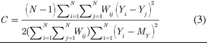
In Equation 3, N is the number of observations (or the geographic markets), Yi and Yj the average office sizes of a geographic markets i and j respectively, and M the mean of average office sizes in all geographic markets. Here Wij is the entry in the contiguity matrix, whose value is 1 if two geographic markets are spatially adjacent to each other and 0 otherwise. The sample Geary’s C is 1.019.
An alternative spatial autocorrelation index is the Moran’s I, as shown in Equation 4 (Griffith, 1987). All terms in the equation are identically defined as in Equation 3:
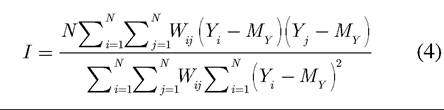
The sample Moran’s I is calculated to be 0.0039. Both the Geary’s C and Moran’s I are asymptotically normally distributed as N increases. Thus they can be tested for significance after converting to standard normal deviates or z scores. Following the procedures defined in Cliff and Ord (1973), the sample Geary’s C and sample Moran’s I are converted to z scores of 0.703 and 0.4457 respectively, both of which are not significant at the 0.05 level. The null hypothesis of non-existence of spatial autocorrelation cannot be rejected. Since the Geary’s C directly compares the difference between adjacent geographic markets while the Moran’s I measures covariance of adjacent geographic markets around a global mean, the former is sensitive to the local spatial autocorrelation while the latter to the global spatial autocorrelation. Thus, the significance test results of both measures confirm at different levels the non-existence of the spatial autocorrelation. As a result, Equation 1 should be used in estimation.
Given a vector of 25 independent variables, a stepwise approach is adopted to select the most suitable variables to enter and retain in the model. This method enters variables one at a time depending on their ability in improving R2 or reducing residuals significantly. The most significant variables are selected before the less significant. Not all selected variables will eventually be retained. Each time a new variable is entered, certain existing variables within the model may become less significant, and thus may be removed from the model. The selection process stops when additional variable cannot improve R2 significantly (Hair, Black, Babin, Anderson & Tatham, 2005). In the end, 7 variables are retained in the model and the results of estimation are shown in Table 2.
Before discussing the estimated results, a brief discussion of the estimation by Hannan and Hanweck (2007) is in order. Of the three variants of their model, R2 ranges from 0.19 to 0.48. The parameter estimate for variable the number of immigrants into a bank market (log form) has a positive sign and is significant at the 0.1 level in all three models. In addition, the parameter estimate for variable the rate of return on interest earning assets (log form) has a negative sign and is significant at the 0.01 level for their second model; and the parameter estimate for variable Herfindahl-Hirschman Index (log form) has a positive sign and is significant at the 0.01 level for their third model. The low R2 and the limited number of significant independent variables of their models provide only limited insight into the determinants of the bank office size, though their models contain very large samples (Observations range from 1386 to 29800).
In comparison, the model in present study reveals much richer information with a higher R2 (0.68) and seven significant independent variables. All parameters retained are significant at the 0.01 level except LogWCAPITAL which is significant at the 0.05 level. A positive parameter estimate for LogINCOME suggests that the average office size increases with the size of the bank geographical market. This result is consistent with the conclusions from Holmes and Stevens (2004) and central place theory that postulate that larger markets are associated with more sophisticated and specialized functions and these specialized functions are provided by larger plants or offices. Although the present study does not directly test
Table 2. Estimation results
| Dependent Variable: LogDepOffice R2=0.68; F=22.056*; Sample size N =84 | ||
| Variable | Parameter | t Value |
| Constant | 1.615 | 1.600 |
| LogINCOME | 0.158** | 3.618 |
| LogHHI | 0.274** | 3.952 |
| LogWHITE | 0.992** | 2.686 |
| LogWINTERNET | 0.230** | 3.099 |
| LogAROA | -0.378** | -2.849 |
| LogCOMMUNITY | -0.225** | -3.331 |
| LogWCAPITAL | -0.231* | -2.568 |
* Significant at the 0.05 level; **significant at the level 0.01
how banking functions differ between markets of different sizes, it seems reasonable to see the large office size as an indication of more sophisticated and specialized banking services.
The positive parameter estimate for LogHHI conforms to expectations, indicating that higher market concentrations bring about larger office sizes within a bank market, in line with the pattern identified by Kim and Vale (2001), and Hannan and Hanweck (2007). This evidence is also consistent with the textbook case of a competitive market where many small players prevail. Here the “small player” literally means physically small offices, though they may be part of larger institutions.
A positive parameter estimate for LogWHITE seems to suggest that in markets with a larger percentage of whites within the population, office sizes tend to be large. This reveals a significant social dimension of bank office size. Within the banking literature, discussions on race and banking are mostly focused on whether or not there are discriminatory practices against racial minorities such as loan denials, higher rates and/or high down-payments, poor services, etc. Evidence here seems to point to the smaller office size as another dimension in racial discrimination in banking. To the extent that racial discrimination in banking exists, as argued by Bradbury, Case and Dunham (1989), Canner and Smith (1991), and Munnell, Browne and McEneraney (1992), smaller bank offices may be indicative of inadequate resources devoted to banking, along with the above mentioned discriminatory practices. To those who reject the existence of systematic discrimination in banking (Benston, Horsky, & Weingartner, 1992; Holmes & Horvits, 1994), smaller offices in markets with concentrated racial minorities may be regarded as a sign of lower end banking and less than specialized service matching the limited banking demand from the racial minorities rather than race-based lending policies. A detailed examination of race and banking along these lines should introduce proxies of banking functions in the model in order to clarify whether the small office size is indeed an indication of limited banking services offered to racial minorities even though they have effective demand for higher-end banking services. An elaborate modeling along these lines is beyond the scope of this study. Nonetheless, evidence here does point to a new dimension of study on race and banking.
A seeming paradox occurs with respect to the effect of using technologies in banking on bank office size. On the one hand, the parameter estimate of LogWCAPITAL has a negative sign, indicating that markets with larger physical capital and premises relative to total bank assets tend to have smaller bank offices. As discussed previously, a high percentage of physical capital and premises in total bank assets are interpreted either as “newness” of the banking sector or as a result of adopting substantial technologies. Either interpretation implies a stronger role for new technologies in banking. Thus this result confirms the expected role of new technology in reducing the bank office size (Hannan & Hanweck, 2007). On the other hand, the parameter estimate of LogWINTERNET has a positive sign, suggesting that markets with higher adoption rates of internet banking tend to have larger office sizes, contrary to general belief about the role of new banking technology in reducing the bank office size.
One possible explanation of this contradiction can be found in the impact of bank market structure on the adoption of different types of banking technologies. According to Allen, Clark, and Houde (2008), when banks can operate through both offline technology within bank offices and online technology such as internet banking or remote deposit, they have incentives to manipulate the relative attractiveness of the two options to encourage customers to adopt the relatively less costly one. The ability of banks to do so depends on market structure. In a competitive market where fierce competition has improved bank office service to a high quality, banks’ preemptive motive of adopting online technology yields to the fear of losing customers to rival banks (business stealing effect) as a result of cutting back on bank office service if online technology is set as priority. The result is to slow internet banking penetration but improve bank office technology. In a concentrated market where each bank faces less competition, the business stealing effect is not as important. As a result, banks expedite adoption of online technology due to the preemptive motive and internet banking penetrates faster and wider than otherwise. Chang (2006) directly associates the adoption of internet banking as a way to provide differentiated banking services, a typical behavior for firms in concentrated markets.
The essential argument here is that the tradeoff between offline technology at bank offices and online technology through internet banking is mediated through market structure. In a study of the adoption of ATMs in banking, Hannan and McDowell (1984) find that banks in concentrated markets are more likely to adopt ATMs than banks in competitive markets. Recent studies on the adoption of internet banking arrive at a similar conclusion (Chang, 2006; Allen, Clark, & Houde, 2008). There has not been empirical research on the diffusion of offline banking technology. However, in studies on the adoption of numerically controlled machine technology by U.S. industries, Mansfield (1968) and Romeo (1977) find that firms in competitive markets are more likely to adopt the new technology. In a recent study on the adoption of a new treatment technology for infertility, Hamilton and McManus (2005) find that the new treatment technology diffuses faster in competitive markets than in concentrated markets. A common characteristic in these examples is that the new technologies are adopted by the firms or clinics at their premises, and thus provide indirect evidence that competitive markets help penetration of offline technology. Anecdotal evidence shows that banks are adopting various technologies to improve competitiveness at bank offices, such as on-site scanning ATMs that reduce the need for tellers (Wilchins & Rauch, 2011), branches with no tellers but with screens connected to tellers at the headquarters (Lariviere, 2012), ATM-teller interfacing facilities allowing partial automation of cash withdrawal transactions and teller multitasking (Adams, 2012), video-conferencing technology that allows a financial expert to work for several offices (Ghaziri, 1998), in-store branches (Hannan & Hanweck, 2007), and increased ratios of financial advising, brokerage and investment experts to tellers and loan officers within the branch network (Kolakowski, 2012).
In the context of the present study, WCAPI- TAL is the percentage of physical capital and premises in the total assets. Since the study uses the percentage of physical capital and premises in total assets as a measure of “newness” in terms of technology, it is reasonable to approximate this percentage as the use of offline banking technology. If small office size is taken as a sign of low market concentration, as discussed previously, the fact that the parameter estimate of LogWCAPITAL is negative can be taken as indirect evidence that in competitive markets, offline banking technologies are invested heavily.
Similarly, WINTERNET measures the percentage of offices in a market that adopt internet banking. The parameter estimate of LogWIN- TERNET is positive, meaning that markets with higher adoption rates of internet banking have large office sizes. Again, if large office size is indicative of concentrated markets, as discussed previously, it would seem logical to see this as indirect evidence that in concentrated markets, online banking technologies have higher penetration rates. In other words, the seemingly contradictory behavior of LogWCAPITAL and LogWINTER- NET may actually indicate the effects of market structure on the adoption of offline and online technologies in banking, consistent with theory and previous study.
It should be noted that this study only finds indirect evidence that market structure has an impact on the adoption of alternative banking technologies. For a true proof, estimation should be done directly between market structure measures and the adoption rates of alternative banking technologies.
The parameter estimate of LogAROA is negative, consistent with a pattern identified by Hannan and Hanweck (2007). This seems to suggest the non-existence of economies of scale at the office level since lower profitability is associated with larger offices. Thus, the use of technology and the non-existence of economies of scale at the office level work together to reduce the size of bank offices in Illinois. That is, the use of technology helps reduce the office size, and a smaller office is not penalized by a lack of economies of scale.
Finally, the parameter estimate for LogCOMMUNITY is negative, indicating that the office size decreases when the number of communities per 10,000 population increases. That is, the presence of many physically separate sub-markets (communities) within a bank geographical market leads to smaller bank offices. Stated another way, the fewer the sub-markets or communities within a geographical market, the larger the bank office size. The point is, physical configuration of local communities within a bank geographical market does matter. It affects the corporate strategy in competing for banking market, and thus affects the banking structure.
While seven independent variables are selected and retained in the model, most variables are not. Specifically, socioeconomic variables such as per capita income, the percentage of population aged between 18 and 65, the percentage of population aged between 16 and 21 who are enrolled in public schools are excluded from the model. All location quotient variables showing economic specialization are also excluded. In addition, population density, the rural-urban dummy variable, and market dynamics variable are also excluded. This suggests that at the level of analysis adopted by this study, not all local geographical characteristics are relevant. However, this does not suggest that these excluded variables are insignificant in shaping bank office sizes under different circumstances.
SUMMARY AND CONCLUDING REMARKS
This study investigates the role of geography in shaping bank office size within Illinois banking, along with technology, economies of scale, and the local bank market conditions. It incorporates a host of proxies for local socioeconomic, demographic, and community characteristics in modeling the bank office size, along with factors such as technology, economies of scale, and local bank market conditions. Although the local bank market conditions are also geographical, they have long been recognized as contributing to the bank office size. The focus of this study is on the local socioeconomic, demographic, and community factors that have not been given sufficient attention in past bank office size modeling. In addition, this study focuses on Illinois banking due to the significant change in the bank office size there in the last few decades. The study also departs from convention by using deposits as a measure of bank office size.
The study finds that geography matters in shaping bank office size. It finds that market size, market concentration, racial composition, and the physical configuration of local communities within a geographical market are factors that affect the bank office size, along with the impacts of banking technology. The roles of market concentration, technology, and economies of scale as determinants of the bank office size have long been known. However, this study also finds the physical configuration of local communities and racial composition within a geographical market are contributors to bank office size. It also confirms the role of the local market size in shaping the bank office size. Specifically, the study finds that bank office size is positively associated with the market size, market concentration, and the percentage of whites within the total population. Bank office size also tends to be larger in markets with a less fragmented physical configuration of local communities. In addition, the study finds that the use of the latest technology in banking may indeed help reduce bank office size. This tendency can be further reinforced by a lack of economies of scale at the bank office level. At the same time, this study finds that the greater adoption of internet banking is associated with larger bank offices. These findings may be taken as indirect evidence that bank market structure has an impact on the adoption of alternative banking technologies. Specifically, in competitive markets, offline banking technologies (or banking at the office) are invested in more heavily while in concentrated markets, online banking technologies have higher penetration rates. The finding that larger offices are associated with higher percentages of white population may be indicative of small bank office size as a form of discrimination in banking against racial minorities, and thus opens up a potentially new dimension in the study of the relationship between race and banking. Finally, finding the non-existence of economies of scale at the bank office level is also significant since it contrasts with existing studies.
A study of determinants of bank office size in Illinois may have relevance to changes in banking in other traditional unit banking states such as Missouri, Kansas, North Dakota, Nebraska, Montana, Oklahoma, Texas, West Virginia, Colorado, Wyoming, Arkansas, Minnesota and Florida. These states have also experienced rapid branch expansion in the last few decades. The average growth of branch offices of all unit banking states (above states plus Illinois) was 1014% between 1980 and 2008 with North Dakota being the lowest at 155% and Wyoming the highest at 6067%. In comparison, the growth in the U.S. as a whole was 114% for the same period. Similarly to Illinois, rapid branch banking developments in these states have occurred only in recent decades. Thus they would be fertile ground for studies that examine how prevailing local conditions and on-going changes help shape the bank office size. However, since market, socioeconomic, and community conditions vary significantly across states, one should expect some of these local conditions to act differently in shaping the bank office size than was found in this study. In particular, given that different states had various banking regulations prior to geographical deregulation, comparison studies may help shed light on the role of banking regulation in affecting the bank office size.
The study of the bank office size has at least two practical implications for U.S. banking in general. First, it may provide insights into banking firms’ future branch strategy. Amid increasing competition in the last three decades and the rapid development of remote banking such as ATMS and especially internet banking, traffic to physical offices has declined over 20% in the past decade. Some industry commentators declared the demise ofbranch offices (Barr, 2010). However, there has been a consensus among most industry analysts that brick and mortar bank offices are here to stay since, despite an exodus of banking transactions toward non-branch options, 80% of sales in banking still occur in branches (EFMA & Microsoft, 2007) and recent surveys show that a majority of people still prefer certain face-to-face interactions with bank staff (Miller, 2011). As a result, the need to combine technology and the face-to-face contacts has become an important debate concerning future branch strategy and bank office design within the banking community. Many envision that future bank offices should move toward being a smaller size, have unconventional interior layouts to create a welcoming atmosphere, have increasing automation of transactional functions, and emphasize sales and advisory functions, etc. (Bills, 2009; Raab, 2009; Adams, 2012).
A study of the determinants of bank office size from a geographical perspective draws attention to geographical factors such as local demographic characteristics, the physical structure of a community, and the hierarchical nature of geographical markets in shaping future branch strategy and bank office design. Geography matters and one format does not fit all. Instead of looking for a single blueprint for an ideal bank office (Sisk, 2009), the branch strategy should place bank offices in an entire banking network and design office functions to cater to varying hierarchical positions in a central place system, different community (sub-market) sizes, and unique community demographic characteristics. In other words, there should be a strategy for the entire office network and a design of a hierarchy of bank offices instead of designing a bank office in isolation. For example, a bank network can be a “hub-and-spoke” type of structure (Adams, 2012), in which small lower level branches function as feeders with no or only a few service staff and highly automated transactional banking (deposit, cash withdrawal, account inquiry, etc.) while larger high level offices at major market centers focus on mid-level decision-making, sales and advising functions mixed with automated transaction banking. At the top of the hierarchy is the flagship office with the top-level decision making, state of the art customer-interactive technology, the whole range of transactional and sales and advisory functions assisted by various combinations of automation.
Another practical implication from the study of bank office size relates to measures of market power, an issue vital in the U.S. antitrust regulation. Most measures of market power currently used are based on the firm level market shares. For example, as discussed previously, the Herfindahl- Hirschman Index or HHI is the sum of squared market shares of all banking firms within a bank market. A higher HHI value means a more concentrated market and thus a higher market power exerted by a smaller number of large firms. Alternative measures use the combined market shares of the top 3 to 5 firms. From a geographical point of view, these measures do not take into account how a bank market is spatially divided among bank branches and how local communities constitute many sub-markets within a bank market. As a result they do not adequately measure the market power associated with a market that is spatial in nature.
Greenhut and Ohta (1975) apply neoclassical price theory in the examination of central placemarket area structure as seen originally in central place theory and prove that it is theoretically equivalent to a monopolistic competitive model developed by Chamberlin (1956). In a standard monopolistic competitive market, sellers compete through providing differentiated products (similar products with slightly different characteristics which help distinguish them). Customers who prefer a particular product are captive to the product and thus are under the monopolistic power of the producer. The source of product differentiation and thus the market power is the set of characteristics of the product. However, when the producer charges too high a price, or a rival producer lowers the price sufficiently, customers may switch to the product offered by the rival producer. In spatial markets where sellers at different central places sell identical product, customers within certain distances of a center are captive to, and thus under the monopolistic power of, the seller due to the longer travel distance (thus the higher cost) to rival sellers further away. Here the source of product differentiation and market power is the location of sellers and distance between sellers. Each seller’s location is unique and the distance from the rival sellers provides cushion against competition. However, too higher a price from the seller or sufficiently lower prices from a rival seller may cause customers to travel to the rival seller.
It is conceivable that as sellers branch out and form additional spatial markets, the size of spatial markets would shrink and so would the spatial monopolistic power since it would now cost less for customers to travel to rival sellers’ markets. The more branch offices there are, the smaller the spatial markets, and the lower the market power each office possesses. In a bank market with two banks, when each operates out of one location, customers can only choose one of the two locations for services. If each bank now operates 10 offices, customers then can obtain services from 20 different locations. Even if each bank applies the same product mix and prices across all of its 10 offices, customers would still have a much easier time choosing between the two sets of product mix and prices than when facing only two locations. The reduced market power by branching directly translates to increased convenience for the customers. Thus market power arises not only from a limited number of firms, but also from a limited number of branch locations. As this study shows, the physical configuration of local communities has an impact on how banking firms establish their branch offices. The conventional measures of market power are based on the notion of a frictionless geographical market, ignoring the monopolistic nature of spatial markets, and leaving out information about community configuration within a bank market. Thus these measures are inadequate. Appropriate measures should incorporate office level information and the community configuration within a bank market.
REFERENCES
ABA Banking Journal. (2011). ABA survey: Popularity of online banking explodes. Retrieved May 10, 2012 from http://www.ababj.com/tech-topics- plus/aba-survey-popularity-of-online-banking- explodes-2293.html
Adams, J. (2012). The shrinking bank branch. American Banker, April 7.
Allen, J., Clark, R., & Houde, J.-F. (2008). Market structure and diffusion of e-commerce: Evidencefrom the retail banking industry (Working Paper: 2008-32). Bank of Canada. Retrieved May 14, 2012 from http://www.econstor.eu/bit- stream/10419/53869/1/584969295.pdf
Anselin, L. (1993). Discrete space autoregressive models. In M. F. Goodchild, B. O. Parks, & L. T. Steyaert (Eds.), Environmental modeling with GIS (pp. 454-469). Oxford University Press.
Avery, R. B., Bostic, R. W., Calem, P. S., & Canner, G. B. (1999). Consolidation and bank branching patterns. Journal of Banking & Finance, 23(2-4), 497-532. doi:10.1016/S0378-4266(98)00094-6
Barr, C. (2010). Whitney sees 5000 bank branches closing. CNN Money. Retrieved May 17, 2012 from http://finance.fortune.cnn.com/2010/11/23/ whitney-sees-5000-bank-branches-closing/
Benston, G. J., Hanweck, G. A., & Humphrey, D. B. (1982). Scale economies in banking: A restructuring and reassessment. Journal of Money, Credit and Banking, 14(4), 435-456. doi:10.2307/1991654
Benston, G. J., Horsky, F., & Weingartner, H. M. (1992). The relationship between the demand and supply of home financing and neighborhood characteristics. Journal of Financial Services Research, 5(3), 72-87. doi:10.1007/BF00115320
Berry, B. J. L., & Parr, J. B. (1988). Market centers and retail location: Theory and applications. Englewood Cliffs, NJ: Prentice Hall.
Bills, S. (2009). Human interaction at a branch: Now on a screen. American Banker, November 17.
Blair, R. D., & Kaserman, D. L. (1985). Antitrust economics. Homewood, IL: Richard D. Irwin Inc.
Bradbury, K. L., Case, K. E., & Dunham, C. R. (1989). Geographic patterns of mortgage lending in Boston, 1982-1987. New England Economic Review, 4, 2-30.
Brevoort, K. P., & Wolken, J. D. (2008). Does distance matter in banking? (Working Paper 2008-34). Board of Governors of Federal Reserve System.
Calomiris, C. W. (2000). U.S. banking deregulation in historical perspective. Cambridge University Press. doi:10.1017/CBO9780511528569 Canner, G. B., & Smith, D. S. (1991). Home mortgage disclosure act: Expanded data on residential lending. Federal Reserve Bulletin, 77, 859-881.
Chamberlin, E. H. (1965). The theory of monopolistic competition. Cambridge, MA: Harvard University Press.
Chang, Y. T. (2006). Dynamic internet banking adoption. (Working Paper: 06-3). University of East Anglia Center for Competition Policy. Retrieved May 14, 2012 from http://papers.ssrn.com/ sol3/papers.cfm?abstract_id=911602
Cliff, A. D., & Ord, J. K. (1973). Spatial autocorrelation. London, UK: Pion Limited.
Contributor. (2009). The branch expansion/remote deposit capture paradox. Retrieved August 10, 2009, from http://www.banktech.com/blog/ar- chives/2009/04/the_branch_expa.html#undefined
Das, A., Ray, S. C., & Nag, A. (2005). Labor-use efficiency in Indian banking: A branch level analysis (Working Paper Series: 2005-4). University of Connecticut Economics Department.
Dick, A. A. (2003). Nationwide branching and its impacts on market structure, quality, and bank performance (Working Paper 2003/35). Board of Governors of Federal Reserve System.
EFMA & Microsoft. (2007). Thefuture role of the “bank store” and its interconnectivity with other channels (A report of the EFMA Banking Advisory Council in partnership with Microsoft). European Financial Market Association and Microsoft.
Federal Reserve System. (2012). Survey of terms of business lending. Retrieved May 20, 2012 from http://www.federalreserve.gov/releases/e2/ current/
Gandhi, D. K., & Swizter, L. N. (1988). Canadian branch banking system: Cost and marketing implications. International Journal of Bank Marketing, 6(4), 55-64. doi:10.1108/eb010838
Gart, A. (1994). Regulation, deregulation, reregulation. New York, NY: John Wiley, and Sons, Inc.
Ghaziri, H. (1997). Information technology in the banking sector: Opportunities, threats, and strategies. Retrieved May 18, 2012 from http:// ddc.aub.edu.lb/projects/business/it-banking.html
Greenhut, M. L., & Ohta, H. (1975). Theory of spatial pricing and market areas. Durham, NC: Duke University Press.
Griffith, D. A. (1987). Spatial autocorrelation: A primer. Washington, DC: AAG.
Guttentag, J. M., & Thomas, K. H. (1979). Branch banking and bank structure: Some evidence from Alabama. Journal of Bank Research, 10, 45-53.
Hair, J. F. Jr, Black, W. C., Babin, B. J., Anderson, R. E., & Tatham, R. L. (2005). Multivariate data analysis. Upper Saddle River, NJ: Pearson/ Prentice Hall.
Hamilton, B. H., & McManus, B. (2005). Technology diffusion and market structure: Evidence from infertility treatment markets (Working Paper). Olin School of Business. Washington University.
Hannan, T. H., & Hanweck, G. A. (2007). Recent trends in the number and size of bank branches: An examination of likely determinants (Working Paper 2008-02). Board of Governors of Federal Reserve System.
Hannan, T. H., & McDowell, J. M. (1984). The determinants of technology adoption: The case of the banking firm. The Rand Journal of Economics, 15(3), 328-335. doi:10.2307/2555441
Hirtle, B. (2007). The impact of network size on bank branch performance. Journal of Banking & Finance, 31(12), 3782-3805. doi:10.1016/j. jbankfin.2007.01.020
Hirtle, B., & Metli, C. (2002). The evolution ofthe U.S. bank branch networks: Growth, consolidation, and strategy. Current Issues in Economics and Finance, 10(8), 1-7.
Holmes, A. L., & Horvitz, P. (1994). Mortgage redlining: Race, risk and demand. The Journal of Finance, 49(1), 81-99. doi:10.1111/j.1540-6261.1994.tb04421.x
Holmes, T. J., & Stevens, J. J. (2004). Geographic concentration and establishment size: Analysis in an alternative economic geography model. Journal of Economic Geography, 4(3), 227-250. doi:10.1093/jnlecg/lbh018
Kim, M., & Vale, B. (2001). Non-price strategic behavior: The case of bank branches. International Journal of Industrial Organization, 19(10), 15831602. doi:10.1016/S0167-7187(00)00064-3
Kolakowski, M. (2012). Trends in branch banking: Implications for bank employments. About.com. Retrieved May 18, 2012 from http://financeca- reers.about.com/od/banker/a/Trends-In-Branch- Banking.htm.
Lariviere, M. (2012). Banking when the teller is in a different town. Operation Room. Retrieved May 18, 2012 from http://operationsroom.wordpress. com/2012/05/17/banking-when-the-teller-is-in- a-different-town/
Lloyd, P., & Dicken, P. (1977). Location in space: theoretical perspectives in economic geography. New York, NY: Harper & Row Publishers.
Longbrake, W. A., & Haslem, J. A. (1975). Production efficiency in commercial banking: The effects of size and legal form of organization on the cost of production of demand deposit services. Journal of Money, Credit and Banking, 7(3), 317-330. doi:10.2307/1991625
Mach, T. L., & Wolken, J. D. (2006). Financial services used by small businesses: Evidence from 2003 survey of small business finances. Federal Reserve Bulletin, 92, 167-195.
Mansfield, E. (1968). Industrial research and technological innovation. New York, NY: Norton.
McCall, A. S. (1980). The impact of bank structure on bank service to local communities. Journal of Bank Research, 101-109.
Miller, J. M. (2011). Face-to-face still trump technology. BankDirect.Com. Retrieved May 15, 2012, from http://www.bankdirector.com/index. php/board-issues/retail/face-to-face-still-trumps- technology/
Munnell, A. H., Browne, L. E., & McEneraney, J. (1992). Mortgage lending in Boston: Interpreting HMDA data (Working Paper: No. 92-7). Federal Reserve Bank of Boston.
Nam, S., & Ellinger, P. N. (2008). Branch expansion of commercial banks in rural America. In Proceedings of the American Agricultural Economics Association Annual Meeting, Orlando, FL.
Nelson, R. W. (1985). Branching, scale economies, and banking costs. Journal of Banking & Finance, 9(2), 177-191. doi:10.1016/0378- 4266(85)90016-0
Orlow, D. K., Radecki, L. J., & Wenninger, J. (1996). Ongoing restructuring of retail banking (Research Paper No. 9634). Federal Reserve Bank of New York.
Raab, M. (2009). Next generation bank branches start taking shape (and size). American Banker, November 4.
Rice, T., & Davis, E. (2007). The branch banking boom in Illinois: A byproduct of restrictive branching laws. Chicago Fed Letter (May).
Romeo, A. A. (1977). The rate of imitation in a capital embodies process innovation. Economica, 44, 63-69. doi:10.2307/2553550
Saidenberg, M. R., & Strahan, P. E. (1999). Are banks still important for financing large businesses? [Federal Reserve Bank of New York.]. Current Issues in Economics and Finance, 5(12), 1-6.
Schuh, S., & Stavins, J. (2008). How consumers pay: Adoption and use of payments (Working Paper No. 12-2). Federal Reserve Bank of Boston.
Sisk, M. (2009). The future of bank branch. American Banker, July 1.
Spieker, R. (2004). Bank branch growth has been steady: Will it continue? In Future of Banking FDIC. Retrieved December 9, 2010, from http:// www.fdic.gov/bank/analytical/future/
Wall Street Journal. (2003). Bank of America bets on customer. October 28.
White Paper. (2011). The branch bank of the future. Hughes Networks Systems. Retrieved May 16, 2012, from http://www.hughes.com/HNS%20 Library%20Presentations%20and%20White%20 Papers/BranchBank_H46930_HR.pdf
Wilchins, D., & Rauch, J. (2012). BofA cuts foretell a downturn in branch banking. Fox Business. September 2011. Retrieved May 18, 2012, from http://novantas.com/news_article.php?id=339
Zardkoohi, A., & Kolari, J. (1992). Branch office economies of scale and scope: Evidence from savings banks in Finland. Journal of Banking & Finance, 18(2), 421-432.
Zhou, B. (2010). Changing retail banking supplydemand mismatch: A tale of two states. International Journal of Applied Geospatial Research, 1(2), 37-54. doi:10.4018/jagr.2010030903
This work was previously published in International Journal of Applied Geospatial Research (IJAGR), 5(1); edited by Donald Patrick Albert, pages 38-59, copyright 2014 by IGI Publishing (an imprint of IGI Global).
APPENDIX
Distortion Using the Hannan and Hanweck Estimation Method
Hannan and Hanweck (2007) use information from County Business Patterns to estimate the number of employees within a county’s banking sector. Their estimation method is discussed in the paper. The potential distortion using their estimation method can be demonstrated as follows. Suppose a size category has the lower bound L and upper bound U. The number of firms in that size category is N. The mid-point of the size category is thus (L+U)∕2 and the total number of employees in the size category, using the Hannan and Hanweck method, is estimated to be N?(L+U)∕2. Now suppose the actual situation is that all firms in the size category have U (number of) employees. Thus the actual total number of employees in the size category is N?U. The Hannan and Hanweck method will under-estimate by N?U-N?(L+U)∕2=N(U-L)∕2. Similarly, if all firms have L (number of) employees, the Hannan and Hanweck method will over-estimate by N(U-L)∕2. Define R=(U-L), the distortion (over-estimation or under-estimation) will be N?R∕2, a product function of N and R. The extent of distortion will rise with the number of firms N within a particular size category and with the size category width R. In other words, the more the firms and the larger the firm size, the more the distortion.
The amount of distortion in the estimations discussed above can be shown in Figure 1, which shows amounts of distortion for size categories 1-4 and 5-9. For a particular size category, the dark line in the middle shows the estimates of the total number of employees for various numbers of firms using the Hannan and Hanweck method. The upper limit shows the actual numbers of employees within the size category if all firms have U (number of) employees. The gray area between the upper limit and the dark
Figure 1. Estimations of the total number of employees and estimation distortions
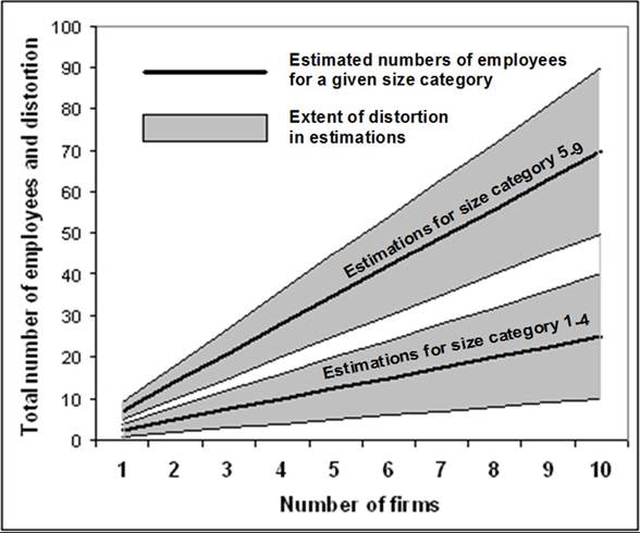
line shows the amount of under-estimation. Similarly, the gray area between the lower limit and the dark line shows the amount of over-estimation when all firms have L (number of) employees. For a particular size category (e.g. 1-4 size category), the gray area fans out, indicating rising distortion with the number of firms. Comparing the 1-4 size category with the 5-9 size category, the gray area for the latter is wider for the same number of firms, indicating larger distortions. The upper and lower limits of the gray area are based on extreme situations where all firms are of the largest or smallest size within a size category. The actual distortion may be smaller since the actual number of employees may fall within the gray area. Nonetheless, the potential distortion is beyond control and there will always be uncertainty regarding the extent of inaccuracy in size estimation.
More on the topic Chapter 63 Does Geography Matter? A Study of Determinants of Bank Office Size in Illinois:
- Chapter 14 Appendix VI: Comments from the Office of Personnel Management
- Chapter Ten: Tony Krone,Corruption and the Rule of Law: A Case Study of Solomon Islands
- APPENDIX TWO The Geography of Ancient Times
- Optimal Muscles to Study for Rest Activity
- B Prohibitions on holding public office
- Congenital Fiber-Type Size Disproportion
- THE RADIUS OF THE DARK-MATTER HALO
- Why do definitions matter?
- The Size and Distribution of the Movements