Space and the global shape of intraspecific competition

Interspecific competition is always closely related to intraspecific competition, so it is logical to begin with a treatment of how spatial patch structure affects the nature of intraspecific competition.

The simplest case to explore is one in which migration is both random and very rare. The within-patch abundances may then be assumed to reach approximately the abundance they would have reached if the patch had been completely isolated.

I consider a multi-patch system having z patches, each obeying the 1-predator-1- prey MacArthur model, with both species potentially present in all patches. This is described by the following equations, where the subscripts denote patch of residence rather than species identity:

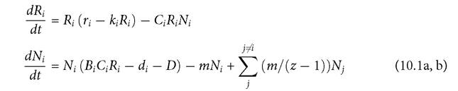
The parameter definitions are identical to those in the equivalent model in previous chapters. All consumers have equal per capita movement rates (m) out of a patch, and all individuals are assumed to survive the dispersal process.

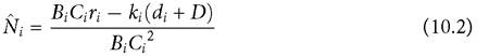
Assuming that the movement rate m is small enough that it does not affect con­sumer abundance appreciably, the following approximation for the abundance of the consumer in patch i can be applied:

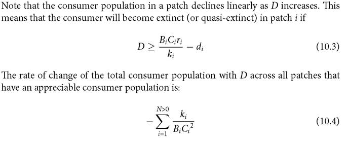
Note that, as the mortality perturbation, D, increases, consumer extinctions occur in the order given by the value of the right-hand side of inequality (10.3); this means that the patches i having the lowest consumer per capita growth rates when the resource is at its carrying capacity will be the first to drop out of the summation in eq. (10.4). These are patches that are characterized by low values of B, C, and/or r as well as those with high values of k_i and/or d_i. High k, low C, and/or low B within a particular patch are all associated with a large change in N_i per unit change in D. Therefore, the consumer extinctions that occur at relatively low mortality perturbations are likely to reduce the total rate of decline of the total N with D by the largest amount. For a simple example, consider two patches that differ only in their values of C, with patch 2 having the smaller C, equal to 1/3 that of patch 1. The smaller capture rate means that the predator goes extinct in an isolated patch 2 at a lower imposed mortality than in patch 1. Patch 2 has a larger rate of decline of N with D than does patch 1. The result of extinction of N₂ is that there is an abrupt decrease in the magnitude of the negative slope of N₁ + N₂ vs D at this point.

The formulas and the 2-patch example just discussed made the simplifying assumption that migration between patches was close to zero. This approximates the case of a very low rate of random movement between patches.

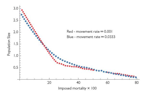
Fig. 10.1 Population size as a function of general mortality applied to the consumers in a 2-patch metacommunity with a single resource and a single consumer species. The parameters are: B₁ = B₂ = 1; C₁ = 1; C₂ = 1/3; r₁ = r₂ = 1; k₁ = 1, k₂ = 1; and d₁ = d₂ = 0.1.

If the above approach is expanded to a system having patches that differ in their values of two or more parameters, the same phenomenon of local consumer extinc­tion occurs, and it causes a similar concave shape of N_totat and D. This phenomenon is similar to what occurs with multi-resource systems in a single patch (see Abrams (2009b) and Chapter 5). If the resources in the individual patches have abiotic growth, the N vs D relationship is concave for a single isolated patch, and the concavi­ty is accentuated by having local consumer extinction with increasing D. If biotic resources have theta-logistic growth with exponents other than 1, the individual seg­ments of the relationship are nonlinear, so the entire relationship becomes more complex in its shape.

Random movement is unlikely in any species that is capable of self-directed travel. Chapter 3 argued that adaptive foraging was prevalent in natural communities, and this is often associated with directed movement. If resources are distinguished both by their physical identity and where they occur, then transfers of both consumers and resources between patches have key roles in determining the strength of indi­rect interactions among different consumers and among different resources. The next two sections consider the major distinguishing features of such movements; whether they are independent of consumer and resource abundances (‘random’) or depend on them in a manner that is adaptive for the moving entity.

10.4