KEY DIAGRAM 8

The misperceptions version of the AD-AS model

The misperceptions ver­sion of the AD-AS model shows how the aggregate demand for output and the aggregate supply of output interact to determine the price level and output in a classical model in which producers misperceive the aggregate price level.

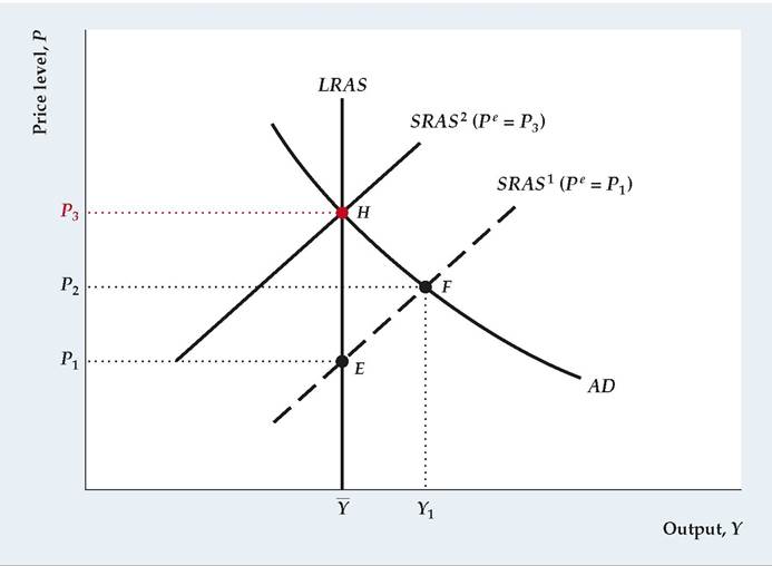
Diagram Elements

■ The price level, P, is on the vertical axis, and the level of output, Y, is on the horizontal axis.

■ The aggregate demand (AD) curve shows the aggre­gate quantity of output demanded at each price level. It is identical to the AD curve in Key Diagram 7 in Chapter 9. The aggregate amount of output demanded is determined by the intersection of the IS and LM curves (see Fig. 9.10). An increase in the price level, P, reduces the real money supply, shifting the LM curve up and to the left and reducing the aggregate quan­tity of output demanded. Thus the AD curve slopes downward.

■ The misperceptions theory is based on the assump­tion that producers have imperfect information about the general price level and hence don't know precisely the relative prices of their products. When producers misperceive the price level, an increase in the general price level above the expected price level fools suppliers into thinking that the relative prices of their goods have increased, so all suppliers increase output. The short-run aggregate supply (SRAS) curve shows the aggregate quantity of output supplied at each price level, with the expected price level held constant. Because an increase in the price level fools producers into supplying more output, the short-run aggregate supply curve slopes upward, as shown by SRAS¹.

■ The short-run aggregate supply curve, SRAS¹, is drawn so that the expected price level, P^e, equals P₁.

■ In the long run, producers learn about the price level and adjust their expectations until the actual price level equals the expected price level. Producers then supply the full-employment level of output, Y, regardless of the price level. Thus the long-run aggre­gate supply (LRAS) curve is vertical at Y = Y, just as in the basic AD-AS model in Key Diagram 7 in Chapter 9.

Factors That Shift the Curves

■ The aggregate quantity of output demanded is deter­mined by the intersection of the IS curve and the LM curve. At a constant price level, any factor that shifts the IS-LM intersection to the right increases the aggre­gate quantity of goods demanded and thus also shifts the AD curve up and to the right. Factors that shift the AD curve are listed in Summary table 14 in Chapter 9.

■ Any factor that increases full-employment output, Y, shifts both the short-run and the long-run aggregate supply curves to the right. Factors that increase full-employment output are listed in Summary table 11 in Chapter 9. An increase in government purchases because it induces workers to supply more labor, also shifts the short-run and long-run aggregate supply curves to the right in the classical model.

■ An increase in the expected price level shifts the short­run aggregate supply curve up.

Analysis

■ The short-run equilibrium is at the intersection of the AD curve and the SRAS curve. For example, if the expected price level is P₁, the SRAS curve is SRAS¹, and the short-run equilibrium is at point P. At F out­put, Y₁, is higher than the full-employment level, Y, and the price level, P₂, is higher than the expected price level, P₁. As producers obtain information about the price level, the expected price level is revised upward, which shifts the SRAS curve up. The long-run equilibrium is at point H, where the long- run aggregate supply (LRAS) curve intersects the AD curve. In the long run (1) output equals Y, and (2) the price level equals the expected price level (both equal P₃). In the long run, when the expected price level has risen to P₃, the short-run aggregate supply curve, SRAS ², passes through H.

►