The Demand for Money
Examine macroeconomic variables that affect the demand for money.
The demand for money is the quantity of monetary assets, such as cash and checking accounts, that people choose to hold in their portfolios.
Choosing how much money to demand is thus a part of the broader portfolio allocation decision. In general, the demand for money—like the demand for any other asset—will depend on the expected return, risk, liquidity, and time to maturity of money and other assets.In practice, two features of money are particularly important. First, money is the most liquid asset. This liquidity is the primary benefit of holding money.8 Second, money pays a low return (indeed, currency pays a zero nominal return). The low return earned by money, relative to other assets, is the major cost of holding money. People's demand for money is determined by how they trade off their desire for liquidity against the cost of a lower return.
In this section we look at how some key macroeconomic variables affect the demand for money. Although we primarily consider the aggregate, or total, demand for money, the same economic arguments apply to individual money demands. This relationship is to be expected, as the aggregate demand for money is the sum of all individual money demands.
The macroeconomic variables that have the greatest effects on money demand are the price level, real income, and interest rates. Higher prices or incomes increase people's need for liquidity and thus raise the demand for money. Interest rates affect money demand through the expected return channel: The higher the interest rate on money, the more money people will demand; however, the higher the interest rate paid on alternative assets to money, the more people will want to switch from money to those alternative assets.
The Price Level
The higher the general level of prices, the more dollars people need to conduct transactions and thus the more dollars people will want to hold.
For example, 65 years ago the price level in the United States was about one-tenth of its level today. Because less money was needed for transactions, the number of dollars that people held in the form of currency or checking accounts—their nominal demand for money—was probably much smaller than the amount of money you hold today. The general conclusion is that a higher price level, by raising the need for liquidity, increases the nominal demand for money. In fact, because prices are ten times higher today than they were in 1950, an identical transaction takes ten times as many dollars today as it did back then. Thus, everything else being equal, the nominal demand for money is proportional to the price level.8Money also has low risk, but many alternative assets (such as short-term government bonds) are not much riskier than money and pay a higher return.
Real Income
The more transactions that individuals or businesses conduct, the more liquidity they need and the greater is their demand for money. An important factor determining the number of transactions is real income. For example, a large, high-volume supermarket has to deal with a larger number of customers and suppliers and pay more employees than does a corner grocery. Similarly, a high-income individual makes more and larger purchases than a low-income individual. Because higher real income means more transactions and a greater need for liquidity, the amount of money demanded should increase when real income increases.
Unlike the response of money demand to changes in the price level, the increase in money demand need not be proportional to an increase in real income. Actually, a 1% increase in real income usually leads to less than a 1% increase in money demand. One reason that money demand grows more slowly than income is that higher-income individuals and firms typically use their money more efficiently. For example, a high-income individual may open a special cash management account in which money not needed for current transactions is automatically invested in nonmonetary assets paying a higher return.
Because of minimumbalance requirements and fees, such an account might not be worthwhile for a lower- income individual.Another reason that money demand grows more slowly than income is that a nation's financial sophistication tends to increase as national income grows. In poor countries people may hold much of their saving in the form of money, for lack of anything better; in richer countries people have many attractive alternatives to money. Money substitutes such as credit cards also become more common as a country becomes richer, again causing aggregate money demand to grow more slowly than income.
Interest Rates
The theory of portfolio allocation implies that, with risk and liquidity held constant, the demand for money depends on the expected returns of both money and alternative, nonmonetary assets. An increase in the expected return on money increases the demand for money, and an increase in the expected return on alternative assets causes holders of wealth to switch from money to higher-return alternatives, thus lowering the demand for money.
For example, suppose that, of your total wealth of $10,000, you have $8000 in government bonds earning 8% interest and $2000 in an interest-bearing checking account earning 3%. You are willing to hold the checking account at a lower return because of the liquidity it provides. But if the interest rate on bonds rises to 10%, and the checking account interest rate remains unchanged, you may decide to switch $1000 from the checking account into bonds. In making this switch, you reduce your holding of money (your money demand) from $2000 to $1000. Effectively, you have chosen to trade some liquidity for the higher return offered by bonds.
Similarly, if the interest rate paid on money rises, holders of wealth will choose to hold more money. In the example, if the checking account begins paying 5% instead of 3%, with bonds still at 8%, you may sell $1000 of your bonds, lowering your holdings of bonds to $7000 and increasing your checking account to $3000.
The sacrifice in return associated with holding money is less than before, so you increase your checking account balance and enjoy the flexibility and other benefits of extra liquidity. Thus a higher interest rate on money makes the demand for money rise.In principle, the interest rate on each of the many alternatives to money should affect money demand. However, as previously noted (see Chapter 4, "In Touch with Data and Research: Interest Rates"), the many interest rates in the economy generally tend to move up and down together. For the purposes of macroeconomic analysis, therefore, assuming that there is just one nominal interest rate, i, which measures the nominal return on nonmonetary assets, is simpler and not too misleading. The nominal interest rate, i, minus the expected inflation rate, πe, gives the expected real interest rate, r, that is relevant to saving and investment decisions, as discussed in Chapter 4.
Also, in reality, various interest rates are paid on money. For example, currency pays zero interest, but different types of checkable accounts pay varying rates. Again for simplicity, let's assume that there is just one nominal interest rate for money, im. The key conclusions are that an increase in the interest rate on nonmonetary assets, i, reduces the amount of money demanded and that an increase in the interest rate on money, im, raises the amount of money demanded.
The Money Demand Function
We express the effects of the price level, real income, and interest rates on money demand as

where
Md = the aggregate demand for money, in nominal terms;
P = the price level;
Y = real income or output;
i = the nominal interest rate earned by alternative, nonmonetary assets;
L = a function relating money demand to real income and the nominal interest rate.
Equation (7.1) holds that nominal money demand, Md, is proportional to the price level, P.
Hence, if the price level, P, doubles (and real income and interest rates don't change), nominal money demand, Md, also will double, reflecting the fact that twice as much money is needed to conduct the same real transactions. Equation (7.1) also indicates that, for any price level, P, money demand depends (through the function L) on real income, Y, and the nominal interest rate on nonmonetary assets, i. An increase in real income, Y, raises the demand for liquidity and thus increases money demand. An increase in the nominal interest rate, i, makes nonmonetary assets more attractive, which reduces money demand.We could have included the nominal interest rate on money, im, in Eq. (7.1) because an increase in the interest rate on money makes people more willing to hold money and thus increases money demand. Historically, however, the nominal interest rate on money has varied much less than the nominal interest rate on nonmonetary assets (for example, currency and a portion of checking accounts always have paid zero interest) and thus has been ignored by many statistical studies of Eq. (7.1). Thus for simplicity we do not explicitly include im in the equation.
An equivalent way of writing the demand for money expresses the nominal interest rate, i, in terms of the expected real interest rate and the expected rate of inflation. Recall from Eq. (2.14) that the expected real interest rate, r, equals the nominal interest rate, i, minus the expected rate of inflation, πe. Therefore the nominal interest rate, i, equals r + πe. Substituting r + πe for i in Eq. (7.1) yields

Equation (7.2) shows that, for any expected rate of inflation, πe, an increase in the real interest rate increases the nominal interest rate and reduces the demand for money. Similarly, for any real interest rate, an increase in the expected rate of inflation increases the nominal interest rate and reduces the demand for money.
Nominal money demand, Md, measures the demand for money in terms of dollars (or yen or euros). But, sometimes, measuring money demand in real terms is more convenient. If we divide both sides of Eq. (7.2) by the price level, P, we get
The expression on the left side of Eq. (7.3), Md ∣P, is called real money demand or, sometimes, the demand for real balances. Real money demand is the amount of money demanded in terms of the goods it can buy. Equation (7.3) states that real money demand, Md/P, depends on real income (or output), Y, and on the nominal interest rate, which is the sum of the real interest rate, r, and expected inflation, πe. The function L that relates real money demand to output and interest rates in Eq. (7.3) is called the money demand function.
Other Factors Affecting Money Demand
The money demand function in Eq. (7.3) captures the main macroeconomic determinants of money demand, but some other factors should be mentioned. Besides the nominal interest rate on money, which we have already discussed, additional factors influencing money demand include wealth, risk, liquidity of alternative assets, and payment technologies. Summary table 9 contains a comprehensive list of variables that affect the demand for money.
Wealth. When wealth increases, part of the extra wealth may be held as money, increasing total money demand. However, with income and the level of transactions held constant, a holder of wealth has little incentive to keep extra wealth in money rather than in higher-return alternative assets. Thus the effect of an increase in wealth on money demand is likely to be small.
Risk. Money usually pays a fixed nominal interest rate (zero in the case of cash), so holding money itself usually isn't risky. However, if the risk of alternative assets such as stocks and real estate increases greatly, people may demand safer assets, including money. Thus increased riskiness in the economy may increase money demand.[117]
| SUMMARY 9 | ||
| Macroeconomic Determinants of the Demand for Money | ||
| An increase in | Causes money demand to | Reason |
| Price level, P | Rise proportionally | A doubling of the price level doubles the |
| Real income, Y | Rise less than | number of dollars needed for transactions. Higher real income implies more transactions |
| proportionally | and thus a greater demand for liquidity. | |
| Real interest rate, r | Fall | Higher real interest rate means a higher re- |
| Expected inflation, πβ | Fall | turn on alternative assets and thus a switch away from money. Higher expected inflation means a lower real |
| Nominal interest rate on | Fall | return on money and thus a switch away from money. Higher return on nonmonetary assets makes |
| nonmonetary assets, i | people less willing to hold money | |
| Nominal interest rate on | Rise | Higher return on money makes people more |
| money, im | willing to hold money. | |
| Wealth | Rise | Part of an increase in wealth may be held in |
| Risk | Rise, if risk of alterna- | the form of money. Higher risk of alternative asset makes money |
| tive asset increases | more attractive. | |
| Fall, if risk of money | Higher risk of money makes it less attractive. | |
| Liquidity of alternative | increases Fall | Higher liquidity of alternative assets makes |
| assets | these assets more attractive. | |
| Efficiency of payments | Fall | People can operate with less money. |
| technologies | ||
However, money doesn't always carry a low risk. In a period of erratic inflation, even if the nominal return on money is fixed, the real return on money (the nominal return minus inflation) may become quite uncertain, making money risky. Money demand then will fall as people switch to inflation hedges (assets whose real returns are less likely to be affected by erratic inflation) such as gold, consumer durable goods, and real estate.
Liquidity of Alternative Assets. The more quickly and easily alternative assets can be converted into cash, the less need there is to hold money. In recent years the joint impact of deregulation, competition, and innovation in financial markets has made alternatives to money more liquid. For example, with a home equity line of credit, a person can now make investments or purchases that are backed by the value of their home. We have mentioned individual cash management accounts whose introduction allowed individuals to switch wealth easily between high-return assets, such as stocks, and more liquid forms. As alternative assets become more liquid, the demand for money declines.
Payment Technologies. Money demand also is affected by the technologies available for making and receiving payments. For example, the introduction of credit cards allowed people to make transactions without money—at least until the end of the month, when payment must be made on the credit card bill. Automatic teller machines (ATMs) probably have reduced the demand for cash because people know that they can obtain cash quickly whenever they need it. In the mid-2000s, check clearing became more efficient, thanks to the Check 21 law, which allowed for electronic clearing of images of checks. This process greatly reduces the costs of clearing checks and allows them to clear much more quickly than before. In the future more innovations in payment technologies, such as the ability to deposit checks and pay for transactions using your phone, undoubtedly will help people operate with less and less cash.[118] Some experts even predict that ultimately we will live in a "cashless society," in which almost all payments will be made through immediately accessible computerized accounting systems and that the demand for cash will be close to zero. The tremendous interest in Bitcoin and other cryptocurrencies in recent years suggests that we are getting closer to a cashless society, though many obstacles remain, especially safety and security issues. See the Application "Bitcoin and Cryptocurrencies."
Application other potential uses in the business world, including "peer-to-peer lending, document verification, ride-sharing and crowdfunding, among other applications."[119]
Are Bitcoin and other cryptocurrencies likely to replace dollars for use in transactions? It may be possible someday, but cryptocurrencies are missing some features of money that people find useful. For something to be useful as money, it needs to serve as a medium of exchange and a store of value. In its medium-of- exchange function, an item that is money should be easy to use to buy things. Originally, Bitcoin seemed to fit that role and a number of merchants agreed to sell their goods in exchange for bitcoins. However, costs of making and validating a Bitcoin transaction are now higher than other payments methods, such as credit cards, so Bitcoin is unlikely to be used for small-value transactions. Also, the security of Bitcoin transactions has not prevented Bitcoin users from suffering large losses, including to hackers and lost password information. In its store-of-value role, for something to be useful as money, its value should be stable. However, Bitcoin's value has risen and fallen dramatically over time, with five days in 2017 in which it fell in value by 20% or more.[120] These fluctuations have led new financial firms to develop another class of cryptocurrency called "stablecoins," which have the goal of creating a cryptocurrency whose value is less volatile and could potentially be used as money.
Someday, we might all use a cryptocurrency in place of dollars. However, there are many obstacles to overcome before that happens. A useful cryptocurrency would have to serve as both a medium of exchange and a store of value, and no cryptocurrency yet does both well.
11See Christopher Koch and Gina C. Pieters, "Blockchain Technology Disrupting Traditional Records Systems," Financial Insights, Federal Reserve Bank of Dallas, Second Quarter 2017.
12See Scott Wolla, "Bitcoin: Money or Financial Investment?" Federal Reserve Bank of St. Louis Page One Economics, March 2018.
rate as a 1% increase in the interest rate is tempting (but incorrect). In fact, it is a 20% increase in the interest rate because 6 is 20% larger than 5.[121] If the interest elasticity of money demand is -0.1, for example, an increase in the interest rate from 5% to 6% reduces money demand by 2% (-0.1 ? 20% = — 2%). Note that, if the interest elasticity of money demand is negative, as in this example, an increase in the interest rate reduces money demand.
What are the actual values of the income elasticity and interest elasticity of money demand? Although the many statistical studies of money demand provide a range of answers, some common results emerge. First, there is widespread agreement that the income elasticity of money demand is positive. For example, in his classic 1973 study of M1 money demand, which established the framework for many later studies, Stephen Goldfeld of Princeton University found this elasticity to be about 2/3.[122] A positive income elasticity of money demand implies that money demand rises when income rises, as predicted by our theory. Goldfeld's finding that the income elasticity of money demand is less than 1.0 is similar to that of many other empirical analyses, although some studies have found values for this elasticity as large as 1.0. An income elasticity of money demand smaller than 1.0 implies that money demand rises less than proportionally with income. Earlier in the chapter we discussed some reasons why, as an individual or nation has higher income, the demand for money might be expected to grow more slowly than income.
Second, for the interest elasticity of money demand, most studies find a small negative value. For example, Goldfeld found the interest elasticity of money demand to be about -0.1 or -0.2. A negative value for the interest elasticity of money demand implies that when interest rates on nonmonetary assets rise, people reduce their holdings of money, again as predicted by the theory.
Finally, Goldfeld's study and others have confirmed empirically that the nominal demand for money is proportional to the price level. Again, this result is consistent with the theory, as reflected in the money demand equation, Eq. (7.3).
Velocity and the Quantity Theory of Money
A concept related to money demand, which at times is used in discussions of monetary policy, is velocity. It measures how often the money stock "turns over" each period. Specifically, velocity is nominal GDP (the price level, P, times real output, Y) divided by the nominal money stock, M. If we let V represent velocity,

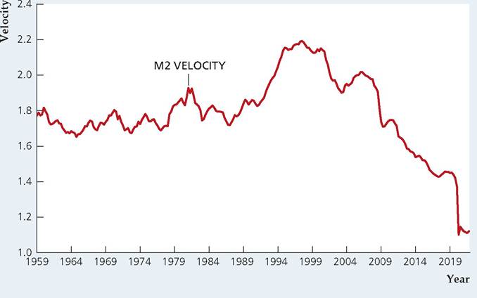
If velocity rises, each dollar of the money stock is being used in a greater dollar volume of transactions in each period, if we assume that the volume of transactions is proportional to GDP. Figure 7.2 shows the velocity of M2 for the United States from 1959 through the fourth quarter of 2021.
FIGURE 7.2
Velocity of M2, 1959Q1-2021Q4
M2 velocity is nominal GDP divided by M2. M2 velocity has trended down since the late 1990s.
Source: Board of Governors of the Federal Reserve System, downloaded from FRED database of the Federal Reserve Bank of St. Louis, fred.stlouisfed.org, series M2SL and GDP.
The concept of velocity comes from one of the earliest theories of money demand, the quantity theory of money.[123] The quantity theory of money asserts that real money demand is proportional to real income, or
where Md/P is real money demand, Y is real income, and k is a constant. In Eq. (7.5) the real money demand function, L (Y, r + πe), takes the simple form kY. This way of writing money demand is based on the strong assumption that velocity is a constant, 1/k, and doesn't depend on income or interest rates.[124]
But is velocity actually constant? As Fig. 7.2 shows, M2 velocity has been unpredictable over short periods and has trended down since reaching a peak in 1998. Throughout the 1990s, people began investing their savings in a broader variety of financial assets than they had before, pulling funds out of bank accounts (which are included in M2) and investing in bonds and stocks (which are not in M2). As a result, demand for M2 at any level of GDP was reduced, raising M2 velocity. Further, when the housing market was booming from the late 1990s to the mid-2000s, funds from refinancing of mortgages were temporarily parked in M2 accounts, leading to increased M2 and lower velocity. Following the pandemic recession, velocity plummeted, as people held increased balances in M2 accounts.
FIGURE 7.3
Growth rates of M2 and nominal GDP, 1960Q1-2021Q4
The growth rates of M2 and nominal GDP plotted here show the percentage increase in both variables from their levels one year earlier, using quarterly data. Growth of M2 has fluctuated considerably because of financial innovations and foreign demand for currency. When the growth rate of the nominal money supply exceeds the growth rate of nominal GDP, velocity declines. Source: Same as for Fig. 7.2.
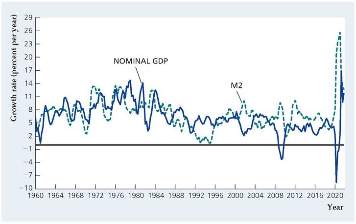
Because velocity is the ratio of nominal GDP to the nominal money supply, the growth rate of velocity equals the growth rate of nominal GDP minus the growth rate of the nominal money supply. Thus when the growth rate of the nominal money supply is lower than the growth rate of nominal GDP, the growth rate of velocity is positive, that is, velocity is rising. Of course when the growth rate of the nominal money supply is higher than the growth rate of nominal GDP, velocity is falling. Figure 7.3 shows the growth rate of nominal GDP as well as the growth rate of nominal M2. As you can see in this figure, the growth rate of M2 has generally exceeded that of nominal GDP since 1998; as a consequence, M2 velocity declined during this period, as shown in Fig. 7.2. The growth rate of nominal M2 was very high following the pandemic recession, far exceeding nominal GDP growth, so M2 velocity fell substantially.
7.4
More on the topic The Demand for Money:
- The Neoclassical Synthesis
- The Monetarist Counter-Revolution
- The Keynesian Revolution
- Article 6.8 Great Portland strikes with convertible bond
- Abel A.B., Bernanke B., Croushore D.. Macroeconomics. 10th Edition, Global Edition. — Pearson,2021. — 690 pp., 2021
- Zimbabwe Village Savings and Loan Associations
- Fligstein Neil. The Banks Did It: An Anatomy of the Financial Crisis. Harvard University Press,2021. — 334 p., 2021
- The Case for Low Interest Rates
- Modern Economics
- CONTENTS