The Dixit-Stiglitz Model and “Aggregate Demand Externalities”

The analysis in the previous section focused on the private and the social values of inno­vations in a partial equilibrium setting. A large part of growth theory is about general equi­librium models of innovation.

can then be embedded in a general equilibrium framework. The most widely-used model of industry equilibrium is the model developed by Dixit and Stiglitz (1977) and Spence (1976), which captures many of the key features of Chamberlin’s (1933) discussion of monopolistic competition. Chamberlin (1933) suggested that a good approximation to the market struc­ture of many industries is one in which each firm faces a downward sloping demand curve (thus has some degree of monopoly power), but there is also free entry into the industry, so that each firm (or at the very least, the marginal firm) makes zero profits.

The distinguishing feature of the Dixit-Stiglitz-Spence model (or Dixit-Stiglitz model for short) is that it allows us to specify a structure of preferences that leads to constant monopoly markups. This turns out to be a very convenient feature in many growth models, though it also implies that this model may not be particularly well suited to situations in which market structure and competition affect monopoly markups. In this section, I present a number of variants of the Dixit Stiglitz model and emphasize its advantages and shortcomings.

12.4.1. The Dixit-Stiglitz Model with a Finite Number of Products. Consider

a static economy that admits a representative household with preferences given by

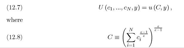
is a consumption index of N differentiated “varieties,” ci,...,cn, of a particular good and y stands for a generic good, representing all other consumption.

More specifically, consider the case in which

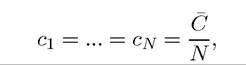
so that the individual purchases a total of C units of differentiated varieties, distributed equally across all N varieties. Substituting this into (12.7) and (12.8),

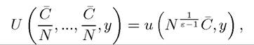
which is strictly increasing in N (since ε > 1) and implies that for a fixed total C units of differentiated commodities, the larger is the number of varieties over which this total number

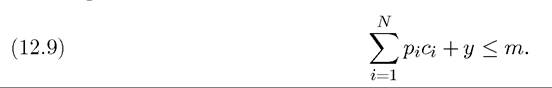
of units are distributed, the higher is the utility of the individual. This is the essence of the love-for-variety utility function. What makes this utility function convenient is not only this feature, but also the fact that individual demands take a very simple isoelastic form. To derive the demand for individual varieties, let us normalize the price of the y good to 1 and denote the price of variety i by pi and the total money income of the individual by m. Then, the budget constraint of the individual takes the form

The maximization of (12.7) subject to (12.9) implies the following first-order condition be­tween varieties: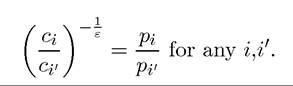

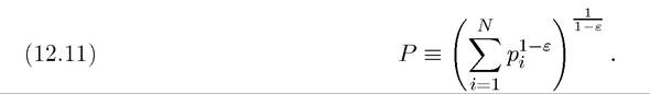
To write this first-order condition in a more convenient form, let P denote the price index corresponding to the consumption index C.

This first-order condition for the consumption index immediately implies that (see Exercise 12.10):

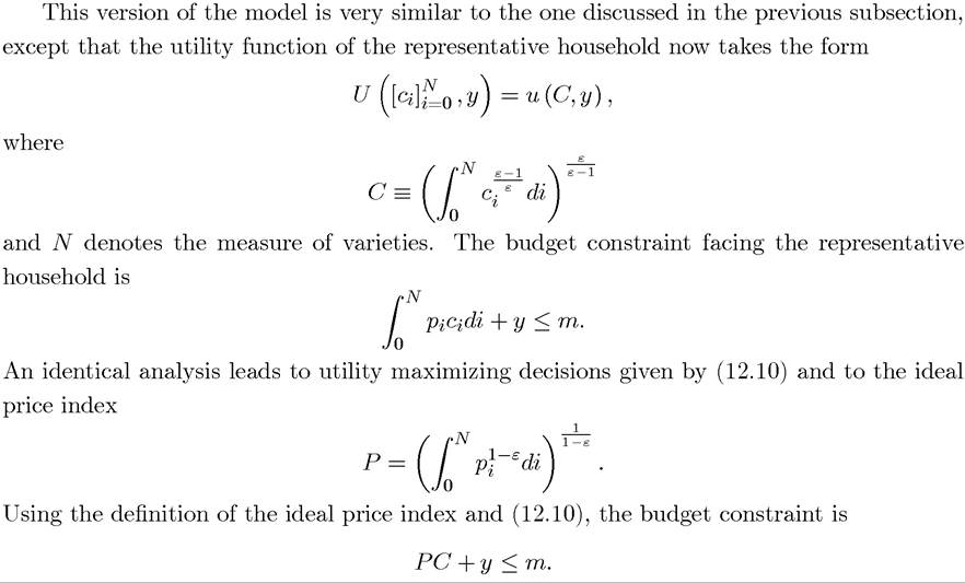
Since P is the price index corresponding to the consumption index C, it is typically referred to as the ideal price index. In many circumstances, it will be convenient to choose this ideal price index as the numeraire. Note, however, that we cannot set this as the price index in this particular instance, since the budget constraint is already in terms of money income, m, and the price of good y is normalized to 1. The choice between C and y is straightforward in this case and boils down to the maximization of the utility function u (C, y) subject to the budget constraint

PC + y ≤ m,

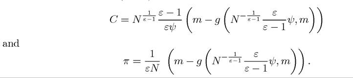
which combines (12.10) and (12.11) with (12.9), in order to obtain a budget constraint ex­pressed in terms of C and y. Now this maximization yields the following intuitive first-order condition: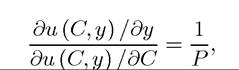

which assumes that the solution is interior, an assumption I maintain throughout this sec­tion to simplify the discussion. The strict joint concavity of u, combined with the budget constraint, implies that this first-order condition can be expressed as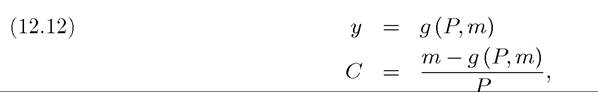

for some function g (∙, ∙).

Next, let us consider the production of the varieties. Suppose that each variety can only be produced by a single firm, who is thus an effective monopolist for this particular commodity. Also assume that all monopolists are owned by the representative household and maximize profits.

Recall that the marginal cost of producing each of these varieties is constant and equal to ψ.

where the term in the first parentheses is c (recall (12.10)) and the second is the difference between price and marginal cost. The complication in this problem comes from the fact that P and C are potentially functions of pi. However, for N sufficiently large, the effect of pi on these can be ignored and the solution to this maximization problem becomes very simple (see Exercise 12.11). This enables us to derive the optimal price in the form of a constant markup over marginal cost:

This result follows because when the effect of firm i^,s price choice on P and C is ignored, the demand function facing the firm, (12.10), is isoelastic with an elasticity ε > 1. Since each firm charges the same price, the ideal price index P can be computed as

Using this expression the profits for each firm are obtained as

Profits are decreasing in the price elasticity for the usual reasons. In addition, profits are increasing in C because this is the total amount of expenditure on these differentiated goods, and they are decreasing in N, since for given C a larger number of varieties means less spending on each variety.

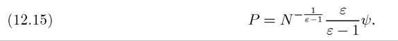
Despite this last effect, the total impact of N on profits can be positive. To see this, let us substitute for P from (12.15) to obtain

It can be verified that depending on the form of the g (∙) function, which in turn depends on the shape of the utility function u in (12.7), profits can be increasing in the number of varieties (see Exercise 12.12).

an aggregate demand externality in the macroeconomics literature. The basic idea is that a higher N raises the utility from consuming each of the varieties because of the love-for- variety effect. The impact of the entry of a particular variety (or the impact of the increase in the production of a particular variety) on the demand for other varieties is a pecuniary externality. This pecuniary externality will play an important role in many of the models of endogenous technological change and we will encounter it again in models of poverty traps in Chapter 21.

12.4.2. The Dixit-Stiglitz Model with a Continuum of Products. As discussed in the last subsection and analyzed further in Exercise 12.12, when N is finite, the equilibrium in which each firm charges the price given by (12.14) may be viewed as an approximation (where each firm only has a small effect on the ideal price index and thus ignores this effect). An alternative modeling assumption would be to assume that there is a continuum of varieties. When there is a continuum of varieties, (12.14) is no longer an approximation. Moreover, such a model will be more tractable because the number of firms, N, need not be a natural number. For this reason, the version of the Dixit-Stiglitz model with a continuum of products is often used in the literature and will also be used in the rest of this book.

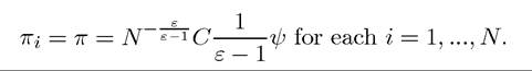
Equation (12.12) then determines ó and C. Since the supplier of each variety is infinitesimal, their price has no effect on P and C. Consequently, the profit-maximizing pricing decision in (12.14) applies exactly, and each firm has profits given by

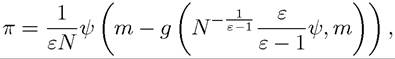
where g (∙) is defined as (12.12) in the previous subsection.

Now using this expression, the entry margin can also be endogenized. Imagine, for exam­ple, that there is an infinite number of potential different varieties, and a particular firm can adopt one of these varieties at some fixed cost μ > 0 and enter the market. Consequently, as in the Chamberlin’s (1933) model of monopolistic competition, in equilibrium all varieties will make zero profits because of free entry. This implies that the following zero-profit condition has to hold for all entrants and thus for all varieties:

1392" class="lazyload" data-src="/files/uch_group77/uch_pgroup317/uch_uch7365/image/image1391.jpg">

As discussed in the next chapter, there is an intimate link between entry by new products (firms) and technological change. Leaving a detailed discussion of this connection to the next chapter, here we can ask a simpler question: do the aggregate demand externalities imply that there is too little entry in a model of this sort? The answer is not necessarily. While the aggregate demand externalities imply that firms do not take into account the positive benefits their entry creates on other firms, the business stealing effect identified above is still present and implies that entry may also reduce the demand for existing products. Thus, in general, whether there is too little or too much entry in models of product differentiation depends on the details of the model and the values of the parameters (see Exercise 12.13).

12.4.3. Objectives of Monopolistic Firms. It is also useful to briefly discuss the objectives of monopolistically competitive firms in the Dixit-Stiglitz model (and related mod­els). Throughout, I follow the industrial organization and the growth literatures and assume that all firms maximize profits, even when they are owned by a “representative household”. One may object to this assumption, noting that, since this is a monopolistically competitive economy where the First Welfare Theorem (e.g., Theorem 5.5) does not hold, the represen­tative household might be made better-off if firms pursued a non-profit maximizing strategy. However, profit maximization is still the right objective function for firms. This is because an allocation in which firms do not maximize profits (instead act in the way that a so­cial planner would like them to act) cannot be an equilibrium. To see this, note that the representative household is itself a price taker—for example, it represents a large number of identical price-taking households. If some firms did not maximize profits, then the households would refuse to hold the stocks of these firms in their portfolios and there would be entry by other profit-maximizing firms instead. Thus, as long as the representative household or the set of households on the consumer side act as price-takers (as has been assumed to be the case throughout), profit maximization is the only consistent strategy for the monopolistically competitive firms.

The only caveat to this arises from a different type of deviation on the production side. In particular, a single firm may buy all of the monopolistically competitive firms and act as the single producer in the economy. This firm might then ensure an allocation that makes consumers better-off relative to the equilibrium allocation considered here. Nevertheless, I ignore this type of deviation for two reasons. First, as usual we are taking the market structure as given, and the market structure here is monopolistic competition not pure monopoly. A single firm owning all production units would correspond to an entirely different market structure, with much less realism and relevance to the issues studied here. Second, in a related model Acemoglu and Zilibotti (1997) show that a single firm owning all production units would not be an equilibrium either because the possibility of free entry would encourage the entry of profit-maximizing firms at the margin, disrupting the equilibrium with the single producer. This is discussed further at the end of Chapter 17. Given these considerations, throughout the book I assume that firms are profit maximizing.

12.4.4. Limit Prices in the Dixit-Stiglitz Model. We have already encountered how limit prices can arise in the previous section, when process innovations are non-drastic relative to the existing technology. Another reason why limit prices can arise is because of the presence of a “competitive” fringe of firms that can imitate the technology of monopolists. This type of competitive pressure from the fringe of firms is straightforward to incorporate into the Dixit-Stiglitz model and will be useful in later chapters as a way of parameterizing competitive pressures.

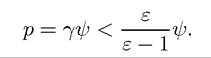
Let us assume that there is a large number of fringe firms that can imitate the technology of the incumbent monopolists. Let us assume that this imitation is equivalent to the pro­duction of a similar good and is not protected by patents. It may be reasonable to assume that the imitating firms will be less efficient than those who have invented the variety and produced it for a while. A simple way of capturing this would be to assume that while the monopolist creates a new variety by paying the fixed cost μ and then having access to a technology with the marginal cost of production of ψ, the fringe of firms do not pay any fixed 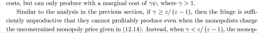olists will be forced to charge a limit price. The same arguments as in the previous section establish that this limit price must take the form

It is then straightforward to see that the entry condition that determines the number of varieties in the market will change to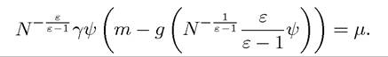

12.4.5. Limitations. The most important limitation of the Dixit-Stiglitz model is the feature that makes it tractable: the constancy of markups as in eq. (12.14). In particular, the model implies that the markup of each firm is independent of the number of varieties in the market. But this is a very special feature. Most industrial organization models imply that markups over marginal cost are declining in the number of competing products (see, for example, Exercise 12.14). While plausible, this makes endogenous growth models less tractable, because in many classes of models, endogenous technological change will correspond to a steady increase in the number of products N. If markups decline towards zero as N increases, this would ultimately stop the process of innovation and thus prevent sustained economic growth. The alternative would be to have a model in which some other variable, perhaps capital, simultaneously increases the potential markups that firms can charge. While such models can be developed, they are more difficult than the standard Dixit-Stiglitz setup. For this reason, the literature typically focuses on Dixit-Stiglitz specifications.

12.5.