Unemployment and Inflation: Is There a Trade-Off?

Describe the Phillips curve relationship between unemployment and inflation.

Newspaper editorials and public discussions about economic policy often refer to the "trade-off" between inflation and unemployment.

The origin of the idea of a trade-off between inflation and unemployment was a 1958 article by economist A. W. Phillips.^[CCXI] Phillips examined 97 years of British data on unemployment and nominal wage growth and found that, historically, unemployment tended to be low in years when nominal wages grew rapidly and high in years when nominal wages grew slowly. Economists who built on Phillips's work shifted its focus slightly by looking at the link between unemployment and inflation—that is, the growth rate of prices—rather than the link between unem­ployment and the growth rate of wages. During the late 1950s and the 1960s, many statistical studies examined inflation and unemployment data for numerous coun­tries and time periods, in many cases finding a negative relationship between the two variables. This negative empirical relationship between unemployment and inflation is known as the Phillips curve.

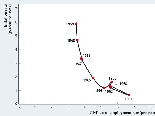
A striking example of a Phillips curve, shown in Figure 12.1, occurred in the United States during the 1960s. The U.S. economy expanded throughout most of the 1960s, with unemployment falling and inflation rising steadily. In Fig. 12.1, the inflation rate is measured on the vertical axis, and the unemployment rate is measured on the horizontal axis. Note that years, such as 1961, that had high unemployment also had low inflation, and that years, such as 1969, that had high inflation also had low unemployment.

FIGURE 12.1

The Phillips curve and the U.S. economy during the 1960s During the 1960s, U.S. rates of inflation and unemployment seemed to lie along a Phillips curve. Inflation rose and unemployment fell fairly steadily during this decade, and policymak­ers apparently had decided to live with higher inflation so as to reduce unemployment.

Source: Bureau of Labor Statistics, downloaded from Federal Reserve Bank of St. Louis FRED database at fred.stlouisfed.org, series CPIAUCSL and UNRATE.

had been published and widely disseminated, was viewed by many as a confirma­tion of his basic finding.

The policy implications of these findings were much debated. Initially, the Phillips curve seemed to offer policymakers a "menu" of combinations of inflation and unemployment from which they could choose. Indeed, during the 1960s some economists argued that, by accepting a modest amount of inflation, macroeco­nomic policymakers could keep the unemployment rate low indefinitely. This belief seemed to be borne out during the 1960s, when rising inflation was accompanied by falling unemployment.

In the following decades, however, this relationship between inflation and unemployment failed to hold: Figure 12.2 shows inflation and unemployment for the period 1970-2021. During those years, unlike the 1960s, there seemed to be no reliable relationship between unemployment and inflation. From the perspective of the Phillips curve the most puzzling period was the mid-1970s, during which the country experienced high inflation and high unemployment simultaneously (stagflation). In 1975, for example, unemployment reached 8.5% of the labor force and the annual inflation rate was 7.1%.

The original empirical results of Phillips and others who extended his work, together with the unexpected experience of the U.S. economy after 1970, raise at least three important questions:

■ Why was the original Phillips curve relationship between inflation and unem­ployment frequently observed historically, as in the cases of Great Britain in the century before 1958 and the United States in the 1960s?

■ Why did the simple negative relationship between inflation and unemploy­ment that seemed to exist during the 1960s in the United States vanish after

FIGURE 12.2

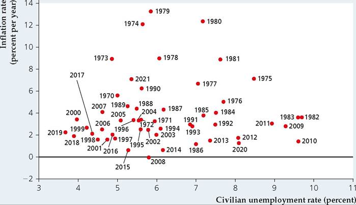
1970? In other words, was there in fact no systematic relationship between inflation and unemployment in the U.S. economy after 1970?

■ Does the Phillips curve actually provide a menu of choices from which policy­makers can choose? For example, by electing to maintain a high inflation rate can policymakers guarantee a permanently low rate of unemployment?

Economic theory provides reasonable answers to these questions; in particu­lar, it explains the collapse of the Phillips curve after 1970. Interestingly, the key economic analysis of the Phillips curve—which predicted that this relationship would not be stable—was done during the 1960s, before the Phillips curve had actually broken down. Thus we have at least one example of economic theorists predicting an important development in the economy that policymakers and the public didn't anticipate.

The Expectations-Augmented Phillips Curve

Although the Phillips curve seemed to describe adequately the unemployment­inflation relationship in the United States in the 1960s, during the second half of the decade some economists, notably Nobel Laureates Milton Friedman^[212] of the University of Chicago and Edmund Phelps^[213] of Columbia University, questioned the logic of the Phillips curve.

Before discussing the significance of their analyses, we need to explain how Friedman and Phelps arrived at their conclusions. To do so we use the extended classical model, which includes the misperceptions theory. (Analytical Problem 3 at the end of the chapter asks you to perform a similar analysis using the Keynesian model.) We proceed in two steps, first considering an economy at full employ­ment with steady, fully anticipated inflation. In this economy, both unanticipated inflation and cyclical unemployment are zero. Second, we consider what happens when aggregate demand growth increases unexpectedly. In this case both positive unanticipated inflation (inflation greater than expected) and negative cyclical unemployment (actual unemployment lower than the natural rate) occur. This outcome demonstrates the Friedman-Phelps point that a negative relationship exists between unanticipated inflation and cyclical unemployment.

We develop the first step of this analysis by using the extended classical model to analyze an economy with steady inflation (see Figure 12.3). We assume that this

FIGUREJ2.3

Ongoing inflation in the extended classical model

If the money supply grows by 10% every year, the AD curve shifts up by 10% every year, from AD¹ in year 1 to AD² in year 2, and so on. If the money supply has been growing by 10% per year for some time and the rate of inflation has been 10% for some time, the expected rate of inflation also is 10%.

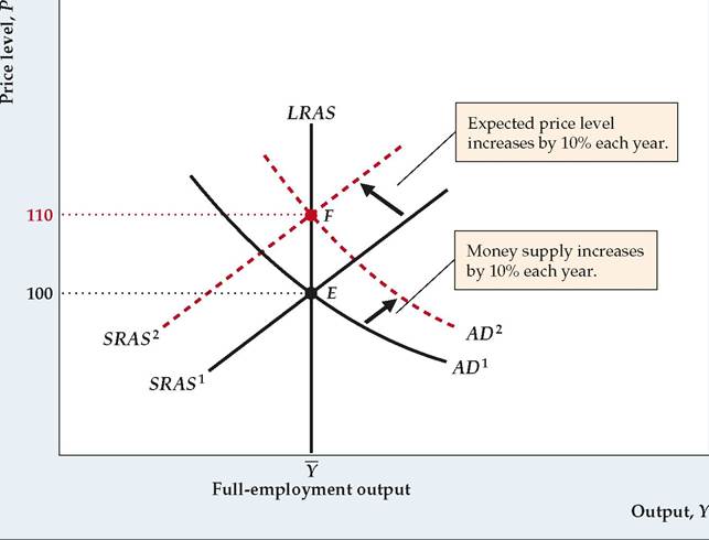
economy is in full-employment equilibrium in which the money supply has been growing at 10% per year for many years and is expected to continue to grow at this rate indefinitely. With the money supply growing by 10% per year, the aggre­gate demand curve shifts up by 10% each year, from AD¹ in year 1 to AD² in year 2, and so on. For simplicity we assume that full-employment output, Y, is constant, but relaxing that assumption wouldn't affect our basic conclusions.

In Fig. 12.3 the short-run aggregate supply (SRAS) curve shifts up by 10% each year. Why? With the growth in money supply fully anticipated, there are no misperceptions. Instead, people expect the price level to rise by 10% per year (a 10% inflation rate), which in turn causes the SRAS curve to shift up by 10% per year. With no misperceptions, the economy remains at full employment with out­put at Y. For example, when the expected price level is 100 in year 1, the short-run aggregate supply curve is SRAS¹. At point E the price level is 100 (the same as the expected price level) and output is Y. In year 2 the expected price level is 110, and the short-run aggregate supply curve is SRAS². In year 2 equilibrium occurs at point F, again with output of Y and equal expected and actual price levels. Each year, both the AD curve and the SRAS curve shift up by 10%, increasing the actual price level and expected price level by 10% and maintaining output at its full­employment level.

What happens to unemployment in this economy? Because output is continu­ously at its full-employment level,, unemployment remains at the natural rate, u. With unemployment at its natural rate, cyclical unemployment is zero. Hence this economy has zero unanticipated inflation and zero cyclical unemployment.

Against this backdrop of 10% monetary growth and 10% inflation, suppose now that in year 2 the money supply grows by 20% rather than by the expected 10% (Figure 12.4). In this case, instead of being 10% higher than AD¹ (as shown

FIGUREJ2.4

Unanticipated inflation in the extended classical model

If the money supply has been growing by 10% per year for a long time and is expected to continue growing by 10%, the expected price level increases by 10% each year. The 10% increase in the expected price level shifts the SRAS curve up from SRAS¹ in year 1 to SRAS² in year 2. Then, if the money supply actu­ally increases by 20% in year 2 rather than by the expected 10%, the AD curve is AD^2,new rather than AD ²,^old. As a result of higher-than-expected money growth, output increases above Y in year 2 and the price level increases to 115, at point G. Because the price level rises by 15% rather than the expected 10%, unan­ticipated inflation is 5% in year 2. This unantici­pated inflation is associ­ated with output higher than Y and unemploy­ment below the natural rate, U (negative cyclical unemployment).

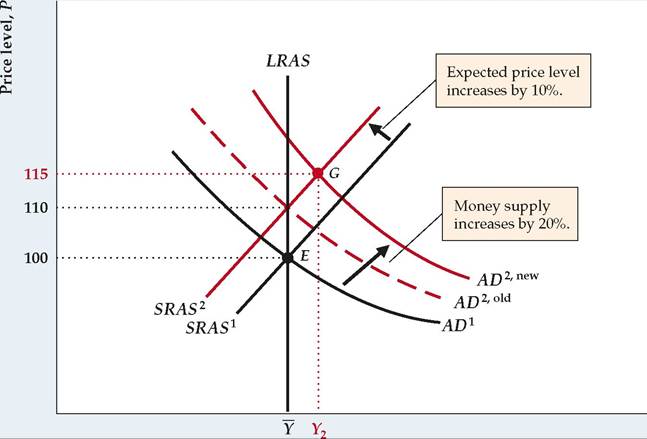
Output, Y

by AD ^2,old), the aggregate demand curve in year 2 will be 20% higher than AD¹ (as shown by AD ^2,new). If this increase in the rate of monetary growth is unanticipated at the beginning of year 2, the expected price level in year 2 remains at 110, and the short-run aggregate supply curve is SRAS², as before. The short-run equilibrium in year 2 is at point G, the intersection of the AD^2,new and SRAS² curves. At G the price level is 115, so the actual rate of inflation in year 2 is 15%. Because the expected rate of inflation was 10%, the 15% inflation rate implies unanticipated inflation of 5% in year 2. Furthermore, because output is above its full-employment level, Y, at G, the actual unemployment rate is below the natural rate and cyclical unem­ployment is negative.

Why is output above its full-employment level in year 2? Note that in year 2 the 15% rate of inflation is less than the 20% rate of money growth but greater than the 10% expected rate of inflation. Because the price level grows by less than does the nominal money supply in year 2, the real money supply, M/P, increases, lowering the real interest rate and raising the aggregate quantity of goods demanded above Y. At the same time, because the price level grows by more than expected, the aggre­gate quantity of goods supplied also is greater than, as producers are fooled into thinking that the relative prices of their products have increased.

Producers can't be fooled about price behavior indefinitely, however. In the long run, producers learn the true price level, the economy returns to full employ­ment, and the inflation rate again equals the expected inflation rate, as in Fig. 12.3. In the meantime, however, as long as actual output is higher than full-employment output, Y, and actual unemployment is below the natural rate, u, the actual price level must be higher than the expected price level. Indeed, according to the misper­ceptions theory, output can be higher than. only when prices are higher than expected (and therefore when inflation is also higher than expected).

Thus in this economy, when the public correctly predicts aggregate demand growth and inflation, unanticipated inflation is zero, actual unemployment equals the natural rate, and cyclical unemployment is zero (Fig. 12.3). However, if aggregate demand growth unexpectedly speeds up, the economy faces a period of positive unanticipated inflation and negative cyclical unemployment (Fig. 12.4). Similarly, an unexpected slowdown in aggregate demand growth could occur, causing the AD curve to rise more slowly than expected; for a time unantici­pated inflation would be negative (actual inflation less than expected) and cycli­cal unemployment would be positive (actual unemployment greater than the natural rate).

The relationship between unanticipated inflation and cyclical unemployment implied by this analysis is

where

π — π^e = unanticipated inflation (the difference between actual inflation, π, and expected inflation, π^e);

= cyclical unemployment (the difference between the actual unemployment rate, u, and the natural unemployment rate, U);

h = a positive number that measures the slope of the relationship between unanticipated inflation and cyclical unemployment.

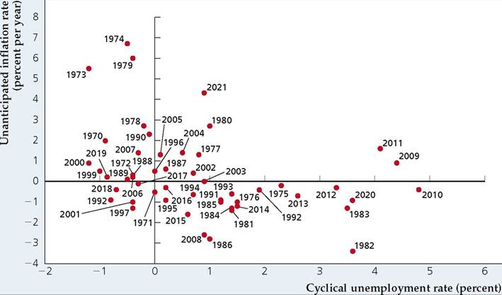
The preceding equation expresses mathematically the idea that unanticipated infla­tion will be positive when cyclical unemployment is negative, negative when cyclical unemployment is positive, and zero when cyclical unemployment is zero.^[215] If we add π^e to both sides of the equation, it becomes

Equation (12.1) describes the expectations-augmented Phillips curve. According to the expectations-augmented Phillips curve, actual inflation, π, exceeds expected inflation, π^e, if the actual unemployment rate, u, is less than the natural rate, U; actual inflation is less than expected inflation if the unemployment rate exceeds the natural rate.

The Shifting Phillips Curve

Let's return to the original Phillips curve, which links the levels of inflation and unemployment in the economy. The insight gained from the Friedman-Phelps analysis is that the relationship illustrated by the Phillips curve depends on the expected rate of inflation and the natural rate of unemployment. If either factor changes, the Phillips curve will shift. To reflect this idea, we call the curve relating the inflation rate to the unemployment rate for a given natural rate of unemploy­ment and expected rate of inflation a short-run Phillips curve.

FIGUREJ2.5

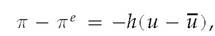
The shifting short­run Phillips curve: an increase in expected inflation

The Friedman-Phelps theory implies that there is a different short-run Phillips curve for every expected inflation rate. For example, PC¹ is the short-run Phillips curve when the expected rate of inflation is 3%. To ver­ify this claim, note from Eq. (12.1) that, when the actual unemployment rate equals the natural rate, u (6% here), the actual inflation rate equals the expected infla­tion rate. At point A, the unemployment rate equals the natural rate and the inflation rate equals 3% on PC¹, so the expected inflation rate is 3% on PC¹. Similarly, at point B on PC², where the unemployment rate equals its natural rate, the inflation rate is 12%, so the expected inflation rate is 12% along PC². Thus an increase in the expected inflation rate from 3% to 12% shifts the short-run Phillips curve up and to the right, from PC¹ to PC².

Changes in the Expected Rate of Inflation. Figure 12.5 shows how a change in the expected inflation rate affects the relationship between inflation and unem­ployment, according to the Friedman-Phelps theory. The curve PC¹ is the short­run Phillips curve for an expected rate of inflation of 3% and a natural rate of unemployment of 6%. What identifies the expected rate of inflation as 3% along PC¹? Equation (12.1) indicates that, when the actual unemployment rate equals the natural rate (6% in this example), the actual inflation rate equals the expected inflation rate. Thus to determine the expected inflation rate on a short-run Phillips curve, we find the inflation rate at the point where the actual unemployment rate equals the natural rate. For instance, at point A on curve PC¹, the unemployment rate equals the natural rate, and the actual and expected rates of inflation both equal 3%. As long as the expected inflation rate remains at 3% (and the natural unemployment rate remains at 6%), the short-run Phillips curve PC¹ will describe the relationship between inflation and unemployment.

Now suppose that the expected rate of inflation increases from 3% to 12%. Figure 12.5 shows that this 9 percentage point increase in the expected rate of infla­tion shifts the short-run Phillips curve up by 9 percentage points at each level of the unemployment rate, from PC¹ to PC². When the actual unemployment rate equals the natural rate on PC² (at point B), the inflation rate is 12%, confirming that the expected inflation rate is 12% along PC². Comparing PC² and PC¹ reveals that an increase in the expected inflation rate shifts the short-run Phillips curve relationship between inflation and unemployment up and to the right.

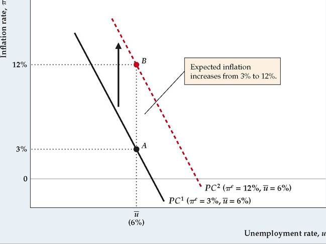
Changes in the Natural Rate of Unemployment. The Phillips curve relation­ship between inflation and unemployment also is shifted by changes in the natural unemployment rate, as illustrated by Figure 12.6. The short-run Phillips curve

FIGUREJ2.6

The shifting short-run Phillips curve: an increase in the natural unemployment rate According to the Friedman-Phelps theory, an increase in the natural unemployment rate shifts the short-run Phillips curve up and to the right. At point A on PC¹, the actual inflation rate and the expected inflation rate are equal at 3%, so the natural unem­ployment rate equals the actual unemployment rate at A, or 6%. Thus PC¹ is the short-run Phillips curve when the natural unemployment rate is 6% and the expected inflation rate is 3%, as in Fig. 12.5. If the natural unemployment rate increases to 7%, with expected inflation unchanged, the short-run Phillips curve shifts to PC³. At point C on PC³, both expected and actual inflation equal 3%, so the natural unemployment rate equals the actual unemployment rate at C, or 7%.

PC¹ shows a natural unemployment rate at 6% and an expected inflation rate at 3% (PC¹ in Fig. 12.6 is the same as PC¹ in Fig. 12.5). Now suppose that the natural unemployment rate increases to 7% but that the expected inflation rate remains unchanged at 3%. As Fig. 12.6 shows, the increase in the natural unemployment rate causes the short-run Phillips curve to shift, from PC¹ to PC³.

To confirm that the natural unemployment rate corresponding to short-run Phillips curve PC³ in Fig. 12.6 is 7%, look at point C on PC³: At C, where the actual and expected inflation rates are equal, the unemployment rate is 7%. Thus the natural unemployment rate associated with short-run Phillips curve PC³ is 7%. This example illustrates that—like an increase in expected inflation—an increase in the natural unemployment rate causes the short-run Phillips curve relationship between inflation and unemployment to shift up and to the right.

Supply Shocks and the Phillips Curve. The Friedman-Phelps theory holds that changes in either expected inflation or the natural unemployment rate will shift the short-run Phillips curve. One type of economic disturbance that is likely to affect both factors is a supply shock. Recall that an adverse supply shock causes a burst of inflation, which may lead people to expect higher inflation.^[216] An adverse supply shock also tends to increase the natural unemployment rate, although the reasons for this effect are different in the classical and Keynesian models.

Recall that, from the classical perspective, an adverse supply shock raises the natural rate of unemployment by increasing the degree of mismatch between workers and jobs. For example, an oil price shock eliminates jobs in heavy-energy­using industries but increases employment in energy-providing industries.

In the Keynesian model, recall that much of the unemployment that exists even when the economy is at the full-employment level is blamed on rigid real wages. In particular, if the efficiency wage is above the market-clearing real wage, the amount of labor supplied at the efficiency wage will exceed the amount of labor demanded at that wage (Fig. 11.2), leading to persistent structural unemploy­ment. An adverse supply shock has no effect on the supply of labor,^[217] but it does reduce the marginal product of labor and thus labor demand. With a rigid effi­ciency wage, the drop in labor demand increases the excess of labor supplied over labor demanded, raising the amount of unemployment that exists when the econ­omy is at full employment. Thus as in the classical model, the Keynesian model predicts that an adverse supply shock will raise the natural unemployment rate.

Because adverse supply shocks raise both expected inflation and the natural unemployment rate, according to the Friedman-Phelps analysis they should cause the short-run Phillips curve to shift up and to the right. Similarly, beneficial sup­ply shocks should shift the short-run Phillips curve down and to the left. Overall, the short-run Phillips curve should be particularly unstable during periods of supply shocks.

The Shifting Short-Run Phillips Curve in Practice. Our analysis of the shifting short-run Phillips curve (Figs. 12.5 and 12.6) helps answer the basic questions about the Phillips curve raised previously in the chapter. The first question was: Why did the original Phillips curve relationship between inflation and unemployment apply to many historical cases, including the United States during the 1960s? The Friedman- Phelps analysis shows that a negative relationship between the levels of inflation and unemployment holds as long as expected inflation and the natural unemployment rate are approximately constant. As shown in Fig. 12.9 later in this chapter, the natural unem­ployment rate changes relatively slowly, and during the 1960s it changed very little. Expected inflation probably was also nearly constant in the United States in the 1960s because at that time people were used to low and stable inflation and inflation remained low for most of the decade. Thus not surprisingly, the U.S. inflation and unemployment data for the 1960s seem to lie along a single Phillips curve (Fig. 12.1).

The second question was: Why did the Phillips curve relationship, so appar­ent in the United States in the 1960s, seem to disappear after 1970 (Fig. 12.2)? The answer suggested by the Friedman-Phelps analysis is that, in the period after 1970, the expected inflation rate and the natural unemployment rate varied con­siderably more than they had in the 1960s, causing the Phillips curve relationship to shift erratically.

Contributing to the shifts of the Phillips curve after 1970 were the two large supply shocks associated with sharp increases in the price of oil that hit the U.S. economy in 1973-1974 and 1979-1980. Recall that adverse supply shocks are likely to increase both expected inflation and the natural rate of unemployment, shifting the Phillips curve up and to the right.

Beyond the direct effects of supply shocks, other forces may have increased the variability of expected inflation and the natural unemployment rate after 1970.

FIGUREJ2.7

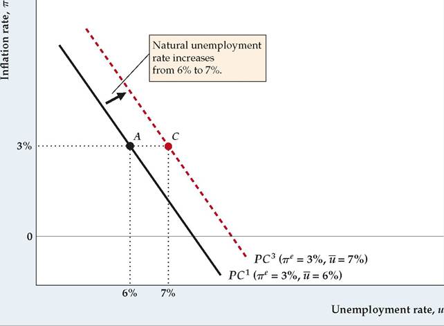
The expectations- augmented Phillips curve in the United States, 1970-2021

The expectations- augmented Phillips curve is a negative relationship between unanticipated inflation and cyclical unemployment. Shown is this relationship for the years 1970-2021 in the United States. Unanticipated inflation equals actual minus expected inflation, where expected inflation in any year is the forecast of CPI inflation from the Livingston Survey. Cyclical unemployment for each year is actual unemployment minus an estimate of the natural unemployment rate for that year (see Fig. 12.9). Note that years in which unanticipated inflation is high usually are years in which cyclical unem­ployment is low.

Source: Bureau of Labor Statistics, downloaded from Federal Reserve Bank of St. Louis FRED database at fred. stlouisfed.org, series CPIAUCSL (inflation) and UNRATE (unemployment rate); expected inflation: Federal Reserve Bank of Philadelphia Livingston Survey at www.philadelphiafed.org/surveys-and- data/real-time-data-research/ livingston-survey; natural rate of unemployment: Congressional Budget Office, downloaded from FRED database, series NROU.

As we discuss later in the chapter, the natural unemployment rate first rose during the 1970s, then fell during the 1980s and 1990s, before leveling off for the first sev­eral years of the 2000s, and then rising after the onset of the Great Recession in 2007.

Expected inflation probably varied more after 1970 because actual inflation varied more (see Fig. 2.4, for the U.S. inflation rate for 1960-2021). After being rela­tively low for a long time, inflation—driven by monetary and fiscal policies that had probably been over-expansionary for several years—emerged as a problem at the end of the 1960s.^[218] The 1970s were a period of high and erratic inflation, the result of the oil price shocks and macroeconomic policies that again were probably too expansionary, especially in the latter part of the decade. In contrast, following the tough anti-inflationary policies of the Federal Reserve during 1979-1982, infla­tion returned to a relatively low level during the 1980s. To the extent that expected inflation followed the path of actual inflation—high and erratic in the 1970s, low in the 1980s—our analysis suggests that the Phillips curve relationship between inflation and unemployment wouldn't have been stable over the period.

Does the unstable Phillips curve during 1970-2021 imply that there was no systematic relationship between inflation and unemployment during that period? The answer is "no." According to the Friedman-Phelps analysis, a negative rela­tionship between unanticipated inflation and cyclical unemployment should appear in the data, even if expected inflation and the natural unemployment rate are changing. Measures of unanticipated inflation and cyclical unemployment for each year during the period 1970-2021 are shown in Figure 12.7. These measures are approximate because we can't directly observe either expected inflation (needed to calculate unanticipated inflation) or the natural unemployment rate (needed to find cyclical unemployment). We used the forecast of Consumer Price Index (CPI) inflation from the Federal Reserve Bank of Philadelphia's Livingston Survey to represent expected inflation for each year, and we used estimates of the natural unemployment rate presented later in the chapter in Fig. 12.9.

Figure 12.7 suggests that, despite the instability of the traditional Phillips curve relationship between inflation and unemployment, a negative relationship between unanticipated inflation and cyclical unemployment did exist during the period 1970-2021, as predicted by the Friedman-Phelps analysis (compare Fig. 12.7 to Fig. 12.2). In particular, note that inflation was much lower than expected and that cyclical unemployment was high during 1982 and 1983, both years that followed Fed Chairman Paul Volcker's actions to reduce inflation through tight monetary policy. Note that one particular point that does not fit the Phillips curve well is the point for 2021, as the aftermath of the pandemic recession in 2020 led to both high inflation and positive cyclical unemployment.

12.2