Moving Linguistic Borders

From a geographical point of view, linguistic displacement can also take place in different ways. For example, when an incoming new elite takes the ruling power of the region, a possible pattern may be the apparition of several language shift sources —e.g., near government, education or religious emplacements.

We can mathematically model the progress of a linguistic frontier over time and space, when the displacement mechanism is due to language acquisition rather than population substitution, with a reaction-diffusion model similar the wave-of-advance models; that is, a model where the population dynamics is sim­plified to short-range migration (e.g., due to marriage), and the increase or decrease in the population number is due to factors such as population growth or conversion into another population group. However, as opposed to the classic wave-of-advance model (Ammerman and Cavalli-Sforza 1973), now the main driver will be the language shift (conversion into another linguistic group) rather than the population growth.

A general reaction-diffusion model to describe the dynamics of two linguistic groups, where a language A is gaining speaker in detriment of language B, may be

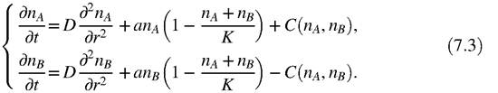
Note that the equations now do not deal with fractions of speakers (p_A and p_B) but with population densities (n_A and n_B).

However, since the introduction of the new language does not yield, in this case, the assimilation of new technologies leading to a rapid population growth, we may assume that the total population number will vary slowly over time, especially in comparison with the language shift rate. Therefore, as a first approximation, the growth term in Eq. 7.3 (second term on the right-hand side) can be dropped. Such approximation simplifies the described dynamics, since now we only have to deal with population diffusion and language shift, but it also allows us to rewrite Eq. 7.3 in terms of the population fraction, thus enabling us to replace the generic con­version term by the language displacement model introduced in the previous sec­tion, Eq.

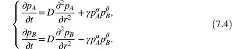
This simplified system describes, for every point in the region, the evolution over time of the fraction of speakers of each language within a population that is not experimenting substantial changes in the total population number. This evolution depends on short-range migrations of the population and the language shift process, according to which the indigenous population acquires a new language that they see as more advantageous socially or economically.

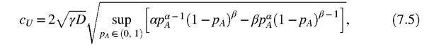
Since we are assuming that the new language is introduced from an adjacent region, the language shift will happen initially near the border, and then the new language will be progressively introduced further into the territory. From the model above, described by Eq. 7.4, we can measure the speed of the linguistic frontier by resolving the equation numerically (that is, with a computational simulation). It is also possible to derive mathematical expressions from which we can obtain a range within which lies the real speed, without having to resort to computational simu­lations. This is possible by assuming that the moving frontier is mostly planar

(which is realistic if the language shift “source” is a political border) and through variational analysis of Eq. 7.4 (Benguria and Depassier 1994, 1998), which leads to the following expression for the upper bound (Isern and Fort 2014)

and the following one for the lower bound (Isern and Fort 2014)

where the gamma function is defined by the following integral

r(x) = J₀°° t^{x — 1} e ^— ‘dt, for x >0 (Murray and Liu 1999).

The values of the bounds are obtained from the previous Eqs. 7.5 and 7.6 by searching for the maximum result of the right-hand side expression for values of S in the range (0, 1) for the lower bound, and for values of p_A in the range (0, 1) for the upper bound.

7.5