Growth with expanding variety

In this section, we present the benchmark model of endogenous growth with expanding variety, and some extensions that will be developed in the following sections.

2.1. Thebenchmarkmodel

The benchmark model is a simplified version of Romer (1990), where, for simplicity, we abstract from investments in physical capital.

The representative household sets a consumption plan to maximize utility, subject to an intertemporal budget constraint and a No-Ponzi game condition. The consumption plan satisfies a standard Euler equation:

There is no physical capital, and savings are used to finance innovative investments.

The production side of the economy consists of two sectors of activity: a competitive sector producing a homogeneous final good, and a non-competitive sector producing differentiated intermediate goods. The final-good sector employs labor and a set of in­termediate goods as inputs. The technology for producing final goods is represented by the following production function:

where xj is the quantity of the intermediate good j, A_t is the measure of intermedi­ate goods available at t, L_y is labor and α ∈ (0, 1). This specification follows Spence (1976), Dixit and Stiglitz (1977) and Ethier (1982). It describes different inputs as im­perfect substitutes, which symmetrically enter the production function, implying that no intermediate good is intrinsically better or worse than any other, irrespective of the time of introduction.

The intermediate good sector consists of monopolistically competitive firms, each producing a differentiated variety j. Technology is symmetric across varieties: the pro­duction of one unit of intermediate good requires one unit of final good, assumed to be the numeraire.^[41] In addition, each intermediate producer is subject to a sunk cost to design a new intermediate input variety. New designs are produced instantaneously and with no uncertainty. The innovating firm can patent the design, and acquire a perpetual monopoly power over the production of the corresponding input.

In the absence of intellectual property rights, free-riding would prevent any innovative activity. If firms could costlessly copy the design, competition would drive ex-post rents to zero. Then, no firms would have an incentive, ex-ante, to pay a sunk cost to design a new input.

The research activity only uses labor. An important assumption is that innovation generates an intertemporal externality. In particular, the design of a (unit measure of) new intermediate good requires a labor input equal to 1∕(δA_t). The assumption that labor productivity increases with the stock of knowledge, A_t, can be rationalized by the idea of researchers benefiting from accessing the stock of applications for patents, thereby obtaining inspiration for new designs.

The law of motion of technical knowledge can be written as:

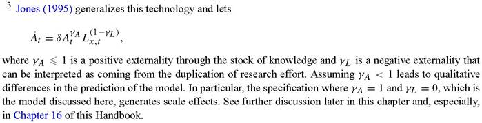
where δ is a parameter and L_x denotes the aggregate employment in research. The rate of technological change is a linear function of total employment in research.³ Finally, feasibility requires that L f L_xyt + L_yyt.

First, we characterize the equilibrium in the final good sector.

The first-order conditions yield the following factor demands: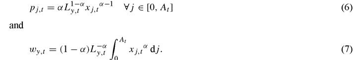

The right-hand side expression is the marginal cost of innovation, independent of At, due to the cancellation of two opposite effects. On the one hand, labor productivity and, hence, the equilibrium wage grow linearly with A_t. On the other hand, the productivity of researchers increases with A_t, due to the intertemporal knowledge spillover. Thus, the unit cost of innovation is constant over time. Note that, without the externality, the cost of innovation would grow over time, and technical progress and growth would come to a halt, like in the neoclassical model.

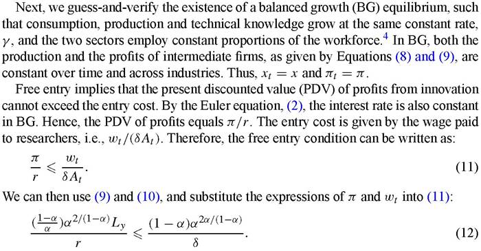
For innovation to be positive, (12) must hold with equality. We can use (i) the resource constraint, implying that L_y = L — L_x, and (ii) the fact that, from (4) and BG, L_x = y/8,to express (12) as a relationship between the interest rate and the growth rate:

⁴ The equilibrium that we characterized can be proved to be unique. Moreover, the version of Romer's model described here features no transitional dynamics, as in AK models [Rebelo (1991)].

Equation (13) describes the equilibrium condition on the production side of the econ­omy: the higher is the interest rate that firms must pay to finance innovation expenditure, the lower is employment in research and growth.

Finally, the consumption Euler equation, (2), given BG, yields:

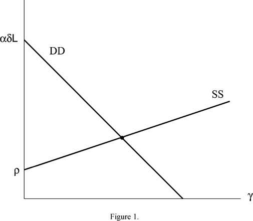
which is the usual positive relation between interest rate and growth. Figure 1 plots the linear equations (13) and (14), which characterize the equilibrium. The two equations correspond, respectively, to the DD (demand for funds) and SS (supply of savings) linear schedules.

An interior solution exists if and only if αδL > ρ. When this condition fails to be satisfied, all workers are employed in the production of consumption goods. When it is positive, the equilibrium growth rate is

showing that the growth rate is increasing in the productivity of the research sector (δ), the size of the labor force (L) and the intertemporal elasticity of substitution of con­sumption (1 /θ), while it is decreasing in the elasticity of final output to labor, (1 — α), and the discount rate.

The trade-off between final production (consumption), on the one hand, and inno­vation and growth, on the other hand, can be shown by substituting the equilibrium expression of x into the aggregate production function, (3). This yields:

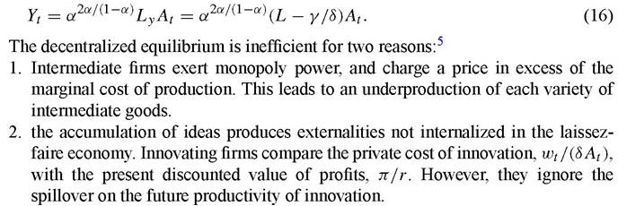
Contrary to Schumpeterian models, innovation does not cause “creative destruction”, i.e., no rent is reduced by the entry of new firms. As a result, growth is always sub- optimally low in the laissez-faire equilibrium. Policies aimed at increasing research activities (e.g., through subsidies to R&D or intermediate production) are both growth- and welfare-enhancing. This result is not robust, however. Benassy (1998) shows that in a model where the return to specialization is allowed to vary and does not depend on firms’ market power (α), research and growth in the laissez-faire equilibrium may be suboptimally too high.

2.2.

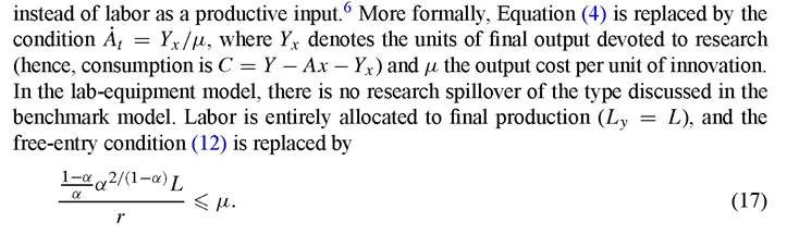
We now consider two alternative specifications of the model that have been used in the literature, and that will be discussed in the following sections. The first specification is the so-called “lab-equipment” model, where the research activity uses final output

⁵ There is an additional reason why, in general, models with a Dixit-Stiglitz technology can generate in­efficient allocations in laissez-faire, namely that the range of intermediate goods produced is endogenous. The standard assumption of complete markets is violated in Dixit-Stiglitz models, because there is no market price for the goods not produced. This issue is discussed in Matsuyama (1995, 1997). A dynamic example of such a failure is provided by the model of Acemoglu and Zilibotti (1997), which is discussed in detail in Section 6.

⁶ The “lab-equipment” model was first introduced by Rivera-Batiz and Romer (1991a); see also Barro and Sala-i-Martin (1995).

Hence, using the Euler condition, (14), we obtain the following equilibrium growth rate:

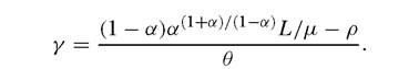
Sustained growth is attained by allocating a constant share of production to finance the research activity.

The second specification assumes that labor is not used in final production, but is used (instead of final output) as the unique input in the intermediate goods production.⁷ More formally, the final production technology is

where Z is a fixed factor (e.g., land) that is typically normalized to unity and ignored. In this model, 1 / A_t units of labor are required to produce one unit of any intermediate input. Therefore, in this version of the model, innovation generates a spillover on the productivity of both research and intermediate production.⁸ We refer to this version as the “labor-for-intermediates” model.

It immediately follows that, in equilibrium, the production of each intermediate firm equals x = L-L_x. The price of intermediates is once more a mark-up over the marginal cost, p_t = w_t/(α A_t). In a BG equilibrium, wages and technology grow at the same rate, hence their ratio is constant. Let ω ? (w_t/A_t). The maximum profit is, then:

The free entry condition can be expressed as:

Clearly, both the “lab-equipment” and “labor-for-intermediates” model yield solutions qualitatively similar to that of the benchmark model.

^[1] We follow the specification used by Young (1993). A related approach, treating the variety of inputs as consumption goods produced with labor, is examined in Grossman and Helpman (1991a).

^[1] The spillover on the productivity of intermediate production is not necessary to have endogenous growth. Without it, an equilibrium can be found in which production of each intermediate falls as A grows: ya = -Yx. In this case, employment in production, Ax, is constant and the growth rate of Y is (1 - a)γA.

2.3. Limitedpatentprotection

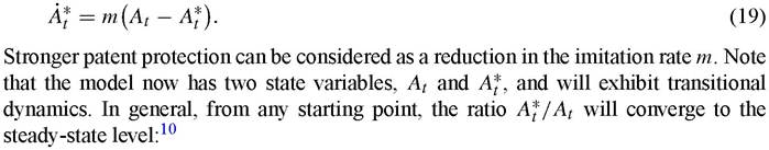
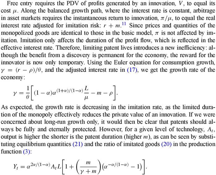
In this section, we discuss the effects of limited patent protection. For simplicity, we focus on the lab-equipment version discussed in the previous section. The expectation of monopoly profits provides the basic incentive motivating investment in innovation; at the same time, monopoly rights introduce a distortion in the economy that raises prices above marginal costs and causes the underprovision of goods. Since the growth rate of knowledge in the typical decentralized equilibrium is below the social optimum, the presence of monopoly power poses a trade-off between dynamic and static efficiency, leading to the question, first studied by Nordhaus (1969a, 1969b), of whether there exists an optimal level of protection of monopoly rights. In the basic model, we assumed the monopoly power of innovators to last forever. Now, we study how the main results change when agents cannot be perfectly excluded from using advances discovered by others. A tractable way of doing this is to assume monopoly power to be eroded at a constant rate, so that in every instant, a fraction m of the monopolized goods becomes competitive.⁹ Then, for a given range of varieties in the economy, A_t, the number of “imitated” intermediates that have become competitive, A*, follows the law of motion:

where γ ? A/A.

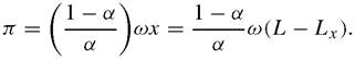
Once a product is imitated, the monopoly power of the original producer is lost and its prices is driven down to the marginal cost by competition. Thus, at each point in time, intermediates still produced by monopolists are sold as before at the markup price 1 /α, while for the others, the competitive price is one. Substituting prices into demand functions yields the quantity of each intermediate sold in equilibrium:

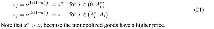
Therefore, a reduction in the patent life entails a trade-off between an immediate con­sumption gain and future losses in terms of lower growth, and its quantitative analysis requires the calculation of welfare along the transition. Kwan and Lai (2003) perform such an analysis, both numerically and by linearizing the BG equilibrium in the neigh­borhood of the steady-state, and show the existence of an optimum patent life. They also provide a simple calibration, using US data on long-run growth, markups and plau­sible values for ρ and θ, to suggest that over-protection of patents is unlikely to happen, whereas the welfare cost of under-protection can be substantial.

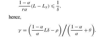
Alternatively, the optimal patent length can be analytically derived in models with a simpler structure. For example, Grossman and Lai (2004) construct a modified version of the model described above, where they assume quasi-linear functions. They show the ^[1] A simple way of seeing this is through the following argument. In a time interval dt, the firm provides a profit stream π ∙ dt, a capital gain of V ∙ dt if not imitated and a capital loss V if imitated (as the value of the patent would drop to zero). In the limit dt → 0, the probability of being imitated in this time interval is m ∙ dt and the probability of not being imitated equals (1 - m ∙ dt). Therefore, the expected return for the firm is π ∙ dt + (1 - m ∙ dt)V ∙ dt - mV ∙ dt. Selling the firm and investing the proceeds in the capital market would yield an interest payment of rV ∙ dt. Arbitrage implies that the returns from these two forms of investment should be equal and in a steady state V = 0, implying π∕V = r + m.

optimal patent length to be an increasing function of the useful life of a product, of con­sumers’ patience and the ratio of consumers’ and producers’ surplus under monopoly to consumers’ surplus under competition. In addition, they derive the optimal patent length for noncooperative trading countries and find that advanced economies with a higher in­novative potential will, in general, grant longer patents. A similar point is made in Lai and Qiu (2003).

3.